Author: Richard Morrill

  • City and Suburb 2010-2013

    Three years is a short time, but perhaps enough to give a sense of what is happening to US metropolitan areas. For both reasons of less uncertainty (and less work for me), I look at just the 107 US metro areas with 500,000 or more people in 2013. These regions house 213 million, two-thirds of the population. I look at the populations of core cities and their suburbs, comparing amounts and rates of change, with further comparison by population size and by region. One definitional problem is what I mean by “core” central city: not the multi-names given by OMB, but rather the historic cities by which we know the places. These can sometimes be a pair, for example, Minneapolis-St. Paul, Dallas-Ft. Worth, San Francisco-Oakland and San Bernardino-Riverside. Another problem I do not try to deal with is whether there were annexations to the core cities in these 3 years.

    City and Suburb: the Nation

    The 107 core cities grew to almost 60 million, but still only 28 percent of the metropolitan population, the suburbs to 153 million. The central cities grew by almost 2 million, a 3.4% gain, while suburbs added 4.4 million, for a slower rate of 3.0%, giving value to the claim of urban revitalization in recent years. We can first deconstruct this change by size of metro areas, large (those over 2.25 million), medium (those from 1 to 2.5 million), and “small” (those under 1 million).

    The interesting story here is that is that the smaller metros, often thought of as the faster growing, e.g., in the 1990s, were the slowest for 2010-2013 at only 2.5%, for both cities and suburbs. Next were the giant metropolises over 2.5 million, growing at an intermediate rate of 3.2%, again with no difference between cities and suburbs. So the particular successful cities now are the medium-sized metros, here from 1 to 2.5 million, whose cities grew by an impressive 4.3% in 3 years, but with a lower 2.3% growth in their suburbs. These intermediate metro areas also had a much smaller suburban share overall of 58% compared to 74% for the largest areas and 69% for the smaller.

    Differences Across Broad Regions, the North, the South and the West

    Confirming expectations, and continuing trends of several decades, the North’s metro areas had the highest total population, but the smallest change for both cities and suburbs, but the region also shows the biggest gap between very low suburban (1.3 %) and a not quite so low city rate of 1.8%. The south, continuing a pattern of larger absolute and relative growth, with city growth moderately faster (5.3%) than in their suburbs (4.6%).  In the west, too, cities grew just slightly more than the suburbs.

    City and Suburb: Population Change 2010-2013 (Thousands)
    Size Large Metros (>2.5 mil) Medium Metros (1-2.5 Mil) Small Metros (Under 1 Mil) Total
    City 2010             31,004                15,557              11,143               57,704
    City 2013             32,016                16,261              11,426               59,703
    Suburb 2010             87,958                34,959              25,738             148,655
    Suburb2013             90,753                35,907              26,368             153,028
    % in suburb 74 69 70 72
    Large Metros (>2.5 mil) Medium Metros (1-2.5 Mil) Small Metros (Under 1 Mil) Total
    Total Change % change Total Change % change Total Change % change Total Change % change
    Metro Change            3,807.0 3.2                 1,624 2.7 914 2.5                 6,345 3.1
    City Change            1,008.0 3.2                    675 4.3 283 2.5                 1,966 3.4
    Suburb Change            2,799.0 3.2                    949 2.3 631 2.5                 4,379 3
    % change in suburbs 74 58 69 69
    Region North South West Total
    City 2010             23,448                17,882              16,358               57,688
    City 2013             23,920                18,866              16,958               59,744
    Suburb 2010             62,910                48,179              37,565             148,654
    Suburb2013             63,732                50,380              38,921             153,033
    % in suburb 73 73 70
    North  South West Total
    Total Change % change Total Change % change Total Change % change Total Change
    Metro Change                1,241 1.4                 3,144 4.7                  1,956 3.6                 6,341
    City Change                   422 1.8                    944 5.3                     600 3.7                 1,966
    Suburb Change                   892 1.3                 2,201 4.6                  1,356 3.6                 4,449
    % change in suburbs 72 70 69


    Example City and Suburb Change

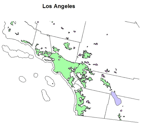
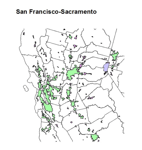
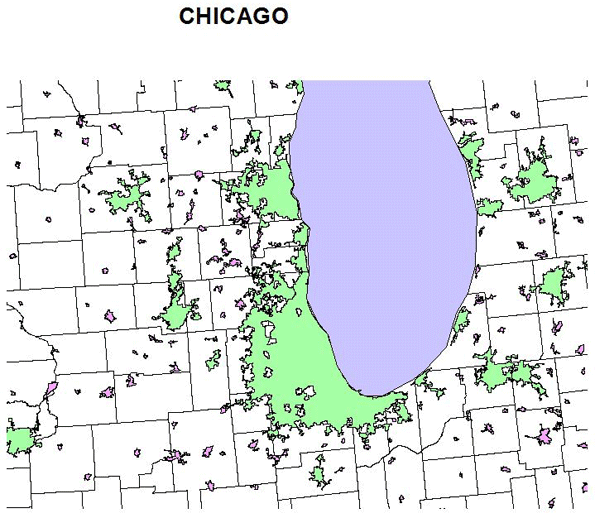
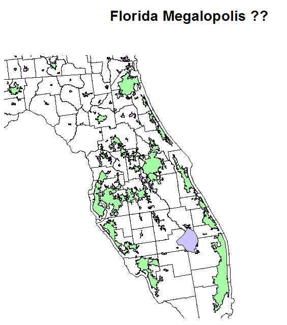
    Here we examine the full list of places, to find which contribute to the growth of cities and of suburbs. I will note metro areas where the highest absolute and relative growth was in cities (1), or in suburbs (2), and those metro areas, where both city and suburban growth were high. But I will also note metro areas with very low growth and then those which are right in the middle, the average place!  Please see the following table.  The reader can also see the geographic patterns of these differences in absolute and relative growth via two maps, the first showing city growth and the second on suburban growth.

    Fast, Slow, and Medium Growth of Cities and Suburbs
    Fast City Growth Fast Suburb Growth Fast City and Suburb Growth
    Rate Rate City Rate Suburb Rate
    Washington 7.4 Houston 7.8 Dallas 6 6
    Atlanta 6.6 Boise 6.1 San Antonio 6.2 6.5
    Seattle 7.2 Des Moines 7.1 Austin 12 7.7
    Charlotte 8.4 Provo 7.1 Orlando 7.2 6.1
    New Orleans 13 Raleigh 6.9 7.7
    Omaha 6.2 Charleston 6.7 7.3
    Durham 7.6 Ft Myers-CapeCoral 7.5 6.6
    Denver 8.2
    Medium City Growth Medium Suburbs
    All 3.3 to 3.5% All 2.8 to 3.2
    Riverside-SanBernardino Minneapolis
    Las Vegas Tampa-St Petersburg
    Provo Baltimore
    Chattanooga Sacramento
    Honolulu Richmond
    Columbia SC Tucson
    Tulsa
    Fresno
    BatonRouge
    Stockton
    Madison
    Slow Growth City Slow Growth Suburb Slow Growth City & Suburb
    Rate Rate City Rate Suburb Rate
    Cincinnati 0.2 Albany 0.7 Chicago 0.9 0.8
    Baltimore 0.2 Dayton 0.2 Detroit -3.5 0.7
    Milwaukee 0.7 Wichita 0.9 St Louis -0.3 0.6
    Birmingham -0.1 New Orleans 0.8 Pittsburgh -0.1 0.2
    Worcester 0.8 Cleveland -1.7 -0.3
    Baton Rouge 0 Providence -0.1 0.2
    Youngstown -1.4 Hartford 0.2 0.2
    Lancaster -1.5 Buffalo -1 0.1
    Portland, ME 0.8 Rochester -0.1 0.4
    New Haven 0.7 -0.1
    Allentown 0.5 0.8
    Akron -0.5 0.7
    Syracuse -0.3 0
    Toledo -1.7 0.9
    Harrisburg -1.4 1.8
    Largest Absolute Growth
    Cities Rate  Absolute Growth Suburbs Rate  Absolute Growth
    New York 2.8                        231,000 New York 13                     153,000
    Dallas 6                        116,000 Los Angeles 2.3                     211,000
    LosAngeles 2.4                          92,000 Dallas 6                     208,000
    Houston 4.1                          95,000 Houston 7.8                     257,000
    San Antonio 6.2                          82,000 Washington 5.3                     266,000
    Austin 12                          95,000 Miami 4.5                     238,000
    Raleigh 6.9                          84,000 Atlanta 4.3                     205,000
    Boston 2.1                     104,000
    SanFrancisco 4                     133,000
    Phoenix 5                     138,000
    Riverside 3.7                     138,000
    Seatttle 4.8                     127,000
    Denver 5.9                     105,000
    Orlando 6.1                     116,000


    City Growth

    Although New York and Los Angeles had high absolute growth, the rates of growth were modest. In contrast, several southern and western cities showed both high numbers and rates of change—notably Austin, Dallas, San Antonio, three just in Texas, and Raleigh, NC. And there were high rates in more southern and western metro areas: Washington, Atlanta, Charlotte, Durham, but especially New Orleans (recovery), and Seattle and Denver, and the northern outlier, Omaha.

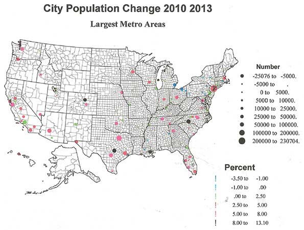
    Most slow-growing or losing cities are in the north – 21 cities – with only Birmingham and Baton Rouge in the south, pretty much a continuation of historic deindustrialization trends. Fourteen have slow growing suburbs as well.

    Suburb Growth

    Suburban growth is absolutely much larger than city growth, so is more prominent on the map.  Fourteen suburban areas added at least 100,000 in three years, led by Washington (266,000), Houston (257,000), and Miami (238,000). But the highest rates of change were for Houston, Des Moines, Boise and Provo, metros where suburban growth was rather faster than central city. Other growing regions include Dallas, San Antonio, Austin, Orlando, Charleston, Raleigh and Ft. Myers-Cape Coral – note all are in the south – for which both city and suburban rates of growth were high.

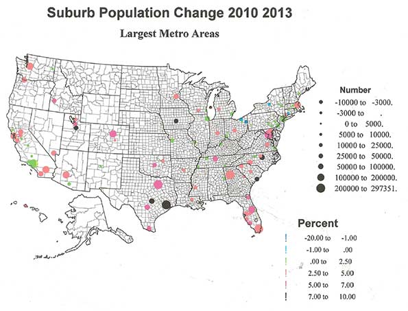
    Slow growing suburbs but not the core cities characterized Atlanta, Dayton, Wichita, and New Orleans, but in 15 other metro areas, all in the north, both suburban and core city growth was slow. Moderately fast (5 to 6%) city growth occurred for San Jose, Nashville, Oklahoma City, McAllen, TX, and El Paso. Moderately fast growing suburban regions include Miami, Phoenix, Denver, Nashville, Jacksonville, Oklahoma City, Salt Lake, and McAllen.     

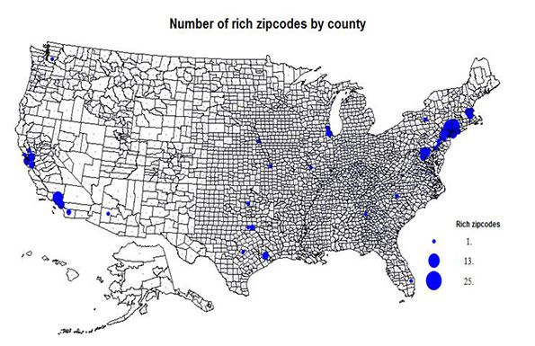
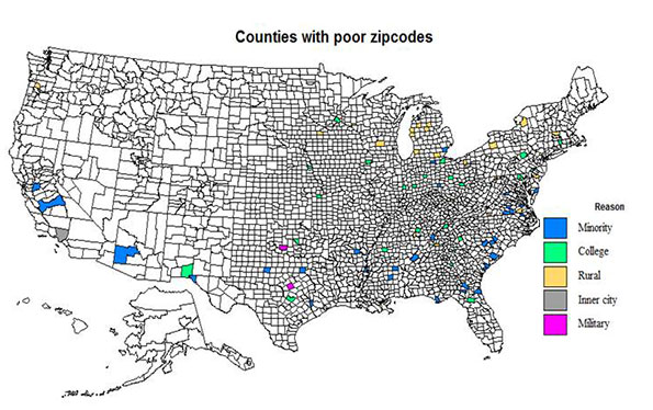
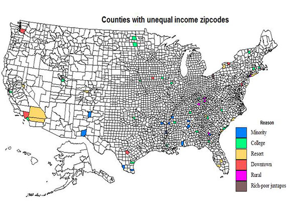
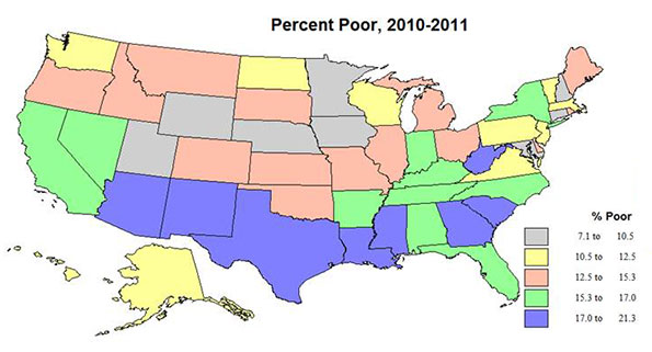
    City and Suburb: Richer and Poorer

    The economic context for cities and suburbs has changed. In the 1970s and 1980s core cities suffered as suburban employment expanded mightily, spurred by the new interstate highways, and also fueled by social change, especially school desegregation, leading to massive white flight. Thus cities became poorer as the more affluent joined the suburban lifestyle. Some cities partly recovered by the late 1980s into the 1990s due to growth of the finance sectors, but suburbanization was still dominant even from 2000 to 2010. But around 1990 some cities – mostly high level regional capitals – began to gentrify, as younger, more affluent, professional and educated, and often unmarried singles or partners, reclaimed desirable older city housing. Some are even reverse commuting to suburban jobs, such as to Microsoft from Seattle.

    Such gentrification led to substantial displacement of the poor and of especially of minorities from the cities to adjacent suburbs, again typified by Seattle experience. The process has gone so far that some central cities are no higher in income and lower in poverty than their suburbs, as in Seattle, San Francisco, and Portland. The most gentrified cities, as measured by the share of neighborhoods upgraded, are Boston, Seattle, New York, San Francisco, Atlanta, Chicago, Portland, Tampa, Los Angeles and Denver—many of the biggest metro areas, and also cities with substantial growth 2010-2013.

    The relative vibrancy and high income of these cities is obviously related as well to the growing inequality of income and wealth of the last 20 years. This has particularly hurt the middle classes, but enabled the educated and professional non-family population to reinvigorate the core cities, even if they have to endure very high housing costs. If the economy improves in terms of jobs and middle class income, I would predict more successful growth in the suburbs than the media and even real estate market folks think, as people find more and more affordable housing available.

    Conclusion

    The period of review is short, but does show continuing growth of both core cities and their suburbs, but with the growth edge going to cities, unlike the dominant pattern of earlier decade. The “new urbanist” interpretation might be that people have come to support denser urban living, but an equally plausible interpretation is that the recession is not yet over, and that the market and financing for suburban single family home living is still suppressed. And a further realistic view is that the huge increase in inequality, reducing the number and buying power of the middle classes, is the more likely explanation of the relative success of cities, as adult children return to family homes, elderly move in with children, or people just double up in homes or are forced to accept living in apartments, even if they might prefer homes.

    Richard Morrill is Professor Emeritus of Geography and Environmental Studies, University of Washington. His research interests include: political geography (voting behavior, redistricting, local governance), population/demography/settlement/migration, urban geography and planning, urban transportation (i.e., old fashioned generalist).

  • Guess What? The Parties are About Even!

    I’ve written extensively about American presidential elections, trying to understand the nature of Democratic success in 2008 and 2012. Many pundits use these elections and changing demographics and public attitudes to write off the future of the Grand Old Party. But this would be a mistake, because we also know that Republicans have a majority in the House of Representatives and in the state legislatures. They also could well get a majority in the US Senate in 2014. Hardly a death spiral.

    Certainly, gerrymandering played a role, and Democrats won a majority of the popular vote for Congress, but the majority was smaller than the margin for president, which was not as large as widely believed, and considerably less than in 2008. Given this confusion it is worth trying to make a more accurate assessment of the D and R balance.  It turns out that there is a peculiar geography of the electorate at all levels and across states, that tends to help Democrats at the statewide level, due to concentrated block voting and concentrations in cities while Republicans, who hold sway over a wider geographic area, at sub-state levels. Obama won 332 electoral votes, 61%, far above his 52% share of the national vote. Democrats won 51 % of the total vote for Congress but won only 200 seats, 46 % of 435, a shortfall of up to 21 seats.

    Besides the votes for president and the House of Representatives in 2012, we can look at the latest result for all 100 Senate seats, for governors of the states, and for all state legislators, in order to get a more honest assessment of Red and Blue America. What states are truly blue or red, and how many are actually more balanced than we might have thought?  Finally it may be useful to compare the actual votes with opinion polls, which seem to show a country somewhat less “liberal” than electoral results. Perhaps voters are a little more liberal than they admit, but let’s see what the fuller set of data show.

    President

    Democrats won 332 electoral votes, 52 or 10% more than their “fair share” of 280  (52% of 538 electors).  The reason for the imbalance is simply that the peculiar geography in 2012 gave the Democrats small margins in some critically large states. For Obama, CA, 55 electoral votes, FL, 29, NY, 29, IL, 20, PA 20, OH, 18, and MI, 16, versus for Romney, TX, 38, GA, 16 and NC, 15. If Romney had carried just the close OH, FL, and PA, he would have won the election!  No wonder Republicans became interested in adopting the Maine and Nebraska allocation of electors by congressional district! However there is no logical basis for allocation by congressional districts, an unrelated office. Rather there is a rational and logical argument to allocate simply by the party shares of the popular vote in states. Table A shows the effect. Obama would have won but by the small margin of 275 to 263 electoral votes, reflecting the actual close division in the electorate.

    Table A
    Electoral Votes 2012 Electoral Votes 2012
      Actual D Electoral Votes Actual R Electoral Votes D If Allocated by Statewide Vote Shares R If Allocated by Statewide Vote Shares
    AL 9 3 6
    AK 3 1 2
    AZ 11 5 6
    AR 6 2 4
    CA 55 33 22
    CO 9 5 4
    CT 7 4 3
    DE 3 2 1
    DC 3 3 0
    FL 29 15 14
    GA 16 7 9
    HI 4 3 1
    ID 3 1 2
    IL 20 12 8
    IN 11 5 6
    IA 6 3 3
    KS 6 2 4
    KY 8 3 5
    LA 8 3 5
    ME 4 2 2
    MD 10 6 4
    MA 11 7 4
    MI 16 9 7
    MN 10 5 5
    MS 6 3 3
    MO 10 4 6
    MT 3 1 2
    NE 5 2 3
    NV 6 3 3
    NH 4 2 2
    NJ 14 8 6
    NM 5 3 2
    NY 29 18 11
    NC 15 7 8
    ND 3 1 2
    OH 18 9 9
    OK 7 2 5
    OR 7 4 3
    PA 20 10 10
    RI 4 3 1
    SC 9 4 5
    SD 3 1 2
    TN 11 4 7
    TX 38 16 22
    UT 6 1 5
    VT 3 2 1
    VA 13 7 6
    WA 12 7 5
    WV 5 2 3
    WI 10 5 5
    WY 3 1 2
    Total 332 205 275 263


    House

    The situation is quite different for Congress (the House), where Republicans won 235 seats to the Democrats 200, while according to the total popular vote, the Democrats would gain a small majority based on their 50.8% share of the total vote,  of 221 to 214 seats (Table B) .  A lot has already been written about this, including charges of theft by gerrymandering. But if we analyze the peculiar geography again carefully, we will find that the net additional seats for the Democrats, if the seats in each state reflected the actual vote, would only be 15, not enough for a majority, simply because so many D votes are “wasted” in safe districts. In 17 states, Democrats won more seats than their share of the vote, 23, but Republicans won 38 “extra” seats in the other 33 states. 

    Table B
    Actual and ideal seats in the House of Representatives
    State Seats in state Ideal D (according to vote share) Actual D Difference Dem %
    CA 53 33 38 5 62%
    NY 27 18 21 3 65%
    MA 9 7 9 2 75%
    IL 18 10 12 2 55%
    MD 8 5 7 2 65%
    CT 5 3 5 2 66%
    NH 2 1 2 1 52%
    AZ 9 4 5 1 46%
    RI 2 1 2 1 59%
    ME 2 1 2 1 62%
    HI 2 1 2 1 67%
    WA 10 5 6 1 54%
    OR 5 3 4 1 58%
    MN 8 5 5 0 56%
    NM 3 2 2 0 55%
    DE 1 1 1 0 66%
    VT 1 1 1 0 76%
    165 100 124 23
    NV 4 2 2 0 50%
    MT 1 0 0 0 45%
    IA 4 2 2 0 52%
    WV 3 1 1 0 40%
    WY 1 0 0 0 26%
    AK 1 0 0 0 31%
    UT 4 1 1 0 33%
    CO 7 3 3 0 49%
    SDS 1 0 0 0 43%
    ND 1 0 0 0 43%
    LA 6 1 1 0 24%
    MS 4 1 1 0 37%
    ID 2 1 0 1 34%
    NJ 12 7 6 1 56%
    GA 14 6 5 1 41%
    KS 4 1 0 1 21%
    WI 8 4 3 1 51%
    NE 3 1 0 1 36%
    AR 4 1 0 1 32%
    TN 9 3 2 1 37%
    KY 6 2 1 1 40%
    MO 8 3 2 1 43%
    AL 7 3 1 2 36%
    OK 5 2 0 2 32%
    SC 7 3 1 2 42%
    IN 9 4 2 2 46%
    MI 14 7 5 2 53%
    TX 36 14 12 2 40%
    VA 11 5 3 2 49%
    NC 13 7 4 3 51%
    FL 27 13 10 3 47%
    OH 16 8 4 4 48%
    PA 18 9 5 4 51%
    US 270 119 77 38 49%


    Note that 54 Democrats won by over 75%, compared to 34 for Republicans. Still, this does leave  probably 8 or 9 districts won by Republicans because of clever gerrymanders, sometimes proudly proclaimed, as in OH and PA, 2 each, and one each in FL, MI, NC,VA and WI, more than offsetting the likely D gerrymander against Republicans in IL. But Democrats would still have lost if there had been no gerrymandering, and the net implication is that the peculiar geography of the Democrat vote means   that it takes at least a 53% total Democratic plurality to win enough of the relatively few close seats to win a majority of the House.

    Senate

    At 2 seats per state regardless of population, Republicans have an inherent advantage to obtain a majority of senators (or governors), since they dominate a majority of states, and Democrats are over-concentrated in a few larger states. The fact that Democrats currently hold 52 of seats plus the support of independents in VT and ME, is a consequence of the timing of Senate elections and perhaps reflects the extremism of some Republican candidates, who alienated enough middle road, independent voters to swing races to the Democrats. It is also significant that in 15 states voters clearly chose to have senators from both  major parties, indicating either that polarization is not so extreme as proclaimed, or that there are a number of closely divided states, that can vote R or D depending on  issues, personalities, and timing. Please see the summary table C for a listing by strength of the D or R votes for senators across the states. The highest D shares (both seats) were in VT, RI, and NY, for Republicans in WY, TN, SD, and ID.

    Governors  

    Republicans hold 29 of the 50 governors, perhaps an underlying indicator of a Republican majority. Yet, from the table you will see that Democrats elected governors in several states that lean Republican overall e.g., MO, AR, MT, and WV, and that there are Republican governors in several states won by Obama, e.g., MI, NV, NM, ME, and NJ. This ambivalence undermines any simple and strict Red versus Blue dichotomy. Many voters are not as utterly polarized as proclaimed. The most extreme Republican votes were in WY, NE, UT LA, and TN, and the highest Democratic shares in DE, NY and yes, AR, which voted only 38% for Obama.

    Legislatures  

    Legislatures are controlled by Republicans in a majority, 26, of states, with Democrats in control in 20 states, with four state divided: Iowa, Kentucky, New Hampshire and Virginia (almost), and even Washington (de facto). The legislatures are overall the most Republican-leaning of the elections analyzed. But even here, the average share of Democrats in legislatures is a respectable 46 percent. The most extremely Republican legislatures are in WY, UT, ID, KS, TN, and SD and the most extremely Democratic are, predictably, in HI, RI, MA, VT and MD. Again in recognition that a simple red and blue dichotomy is not that certain is the fact that in four states, KY, IA, VA, and NH, the legislative houses are split between the parties.

    So what is the best estimate of the real division between Red and Blue America?

    Table C ranks the states by my composite average index based on the races for president, the House of Representatives, state legislatures, US senators and governors. The numbers (percents) are the Democratic share of the vote for president, for the US house, for US senators and for governors, but for state legislatures, the percent shares of legislators who are Democrats. The final column Is a simple average of these five values. In this way I can distinguish those states which are consistently Democrat or Republican, from those which really are less polarized and more balanced.

    TABLE C: Summary of Democratic-Republican Voting Record
    Electoral Votes President %D Congress %D State Legislatures Senators %D Governors %D Number of D Wins Composite Index
    Sen %D House %D Legis Ave. Type
    WY 3 28.8 25.7 13.3 13.3 13.3 25 27 0 24.0 R++
    UT 6 25.4 33.4 17.2 18.7 18.0 34.75 34 0 29.1 R++
    KS 6 38.9 20.9 22.5 26.4 24.5 33.25 36 0 30.7 R++
    ID 4 33.6 33.9 17.1 18.6 17.9 33.5 39 0 31.6 R++
    OK 7 33.2 32.4 25.0 28.7 26.9 35 40 0 33.5 R++
    TN 11 39.6 36.8 21.2 27.6 24.4 34 35 0 34.0 R++
    SD 3 40.8 42.6 20.0 24.3 22.1 31.25 38.5 0 35.0 R++
    NE 5 38.9 35.8 42 27 0 35.9 R+ 
    ND 3 39.9 43.2 28.3 24.5 26.4 36.75 35.5 0 36.3 R+ 
    AL 9 38.8 36.0 25.5 37.1 31.3 35.6 42 0 36.7 R+ 
    LA 8 41.3 23.9 41.0 42.9 41.9 47.5 34 0 37.7 R+ 
    AK 3 42.7 30.9 35.0 37.5 36.3 38.25 41 0 37.8 R+ 
    MS 6 44.2 36.9 36.5 47.9 42.2 40.3 38 0 40.3 R
    GA 16 46.0 40.8 32.1 33.3 32.7 41.75 46 0 41.5 R
    TX 38 42.0 40.0 38.7 36.7 37.7 43.25 45 0 41.6 R
    SC 9 44.7 42.0 39.1 37.7 38.4 38.25 48 0 42.3 R
    IN 11 44.8 45.8 26.0 31.0 28.5 47.25 48.2 0 42.9 R
    AZ 11 45.4 45.6 43.3 40.0 41.7 43.25 45 0 44.2 R
    FL 29 50.4 47.0 35.0 38.3 36.7 40.5 49.3 1 44.8 R
    MO 10 45.2 43.3 29.4 32.5 31.0 49.5 55.5 1 44.9 R
    KY 8 38.5 40.0 40.0 55.0 47.5 45.7 56 1 45.5 R
    NC 15 49.0 50.9 36.0 35.8 35.9 48.5 44.5 1 45.8 R
    OH 18 51.5 47.9 30.3 39.4 34.8 47 49.5 1 46.2 R
    239
    AR 6 37.8 32.3 40.0 49.0 44.5 59.75 64.5 2 47.8 BalR
    MT 3 43.0 44.5 46.0 37.0 41.5 62 50.5 2 48.3 BalR
    WI 10 53.5 50.8 45.5 39.4 42.4 50.5 47 3 48.8 BalR
    PA 20 52.7 50.8 46.0 45.8 45.9 51.5 45.5 3 49.3 BalR
    IA 6 53.0 51.5 52.0 47.0 49.5 48.6 45 2 49.5 BalR
    WV 5 36.3 40.1 70.6 54.0 62.3 57.5 52 3 49.6 BalR
    50
    MI 16 54.8 52.7 31.6 46.4 39.0 61.5 42 3 50.0 BalD
    VA 13 52.0 49.0 50.0 32.0 41.0 59 50.8 3 50.4 BalD
    NH 4 52.8 52.2 45.8 55.3 50.5 45.25 54 4 51.0 BalD
    NV 6 53.4 49.8 52.4 64.3 58.3 50.5 46 3 51.6 BalD
    39
    CO 9 52.7 48.6 54.3 56.9 55.6 52.25 56 4 53.0 D
    NM 5 55.3 55.2 59.5 55.7 57.6 56.5 46.4 4 54.2 D
    ME 4 57.9 61.7 60.0 56.7 58.3 46.5 49 3 54.7 D
    WA 12 57.6 54.4 51.0 56.1 53.6 56.5 51.5 5 54.7 D
    OR 8 56.3 58.0 53.3 57.6 55.5 54.75 50.4 5 55.0 D
    MN 10 53.9 56.3 58.2 54.5 56.3 58.25 50.5 5 55.1 D
    NJ 14 59.0 55.6 60.0 60.0 60.0 58 46 4 55.7 D
    IL 20 58.6 55.4 67.8 60.2 64.0 59.5 50.5 5 57.6 D
    CT 7 58.8 65.5 61.1 64.9 63.0 55.25 50.3 5 58.6 D
    CA 55 61.9 62.0 68.4 70.0 69.2 58.25 53 5 60.9 D+
    MD 10 63.3 65.5 74.5 69.5 72.0 61.25 56 5 63.6 D+
    NY 29 64.3 64.8 52.4 70.5 61.4 67.25 62 5 64.0 D+
    DE 3 59.4 65.8 61.9 65.9 63.9 62.75 70 5 64.4 D+
    RI 4 64.0 59.0 84.2 92.0 88.1 69 53 5 66.6 D++
    MA 11 61.8 74.9 90.0 81.9 85.9 60 52 5 66.9 D++
    VT 3 68.2 75.6 76.7 67.6 72.1 69 51 5 67.2 D++
    HI 4 71.7 67.5 96.0 86.3 91.1 69.3 58 5 71.5 D++
    DC 3 95.0                  
    211


    Overall 23 states with 239 electoral votes lean fairly strongly Republican across the 5 measures, despite Obama carrying FL and OH, and six more states were somewhat balanced, but leaning moderately Republican, with 50 electoral votes. Of these Obama won 3, WI, PA, and VA, but none of the 5 Obama-carried states in these sets can be considered safely Democratic. Seven states had composite indices less than 35% D, a fairly extreme set. Five states were quite Republican with indices 35 to 40 Democratic, and a larger number, 11, were less strongly or consistently Republican (indices 40 to 46}. The six marginally Republican states, with indices 47.8 to 49.6, all have a mixed pattern of Democratic and of Republican majority percents. AR, MT and WV are an interesting subset, with a less “urban liberal” kind of Democratic tradition.

    Seventeen states (plus the District of Columbia) have Democratic indices over 53. With four (RI, VT, HI, MA) and DC in the over 65 set, 4 in the moderately strong D set, 60 to 65, CA, MD, NY, and DE, and then  9 is the group with D indices from 53 to 60.  But note that 4 of these had a Republican majority in some category. The remaining 4 states with indices from 50 to 52, are only marginally D, and indeed are quite mixed across the categories, almost a classic definition of balance. What all the 21 D leaning states have in common is that Obama won them in 2012.

    In summary Republicans are stronger overall in 29 states with 289 electoral votes, to Democrats in 21 states (+DC) with 249 electoral votes. Democrats can overcome this territorial Republicanism only by the peculiar geography of their huge urban vote, which can enable them to carry marginally Republican states.

    Thus, as to the presidential election in 2016, is there hope for the Republicans? I am convinced that there is now a national consensus that the time has come for a woman president, and that Hilary Clinton can match or even beat Obama’s lopsided 2008 victory, because potentially millions of women will defy their husbands and desert their otherwise moderate conservatism and vote for Clinton. Otherwise the Democrats would be in a desperate situation.

    But 2014 is an entirely different proposition. If we ignore the first column (presidential), Republicans are in a very strong position for the Senate, the House, governors, and legislatures.  This outcome is likely, despite the demographic transition from domination by older white males to younger, more liberal, more urban generations. But moderately conservative folk remain the majority, as attested to by the latest national polls. For example, Gallup polls show conservatives at 38%, liberals at 23 (the highest ever but still unimpressive) and moderates at 34%. The Republican failure to take advantage of this inherent moderate majority reflects the problem with reactionary conservatism that enables Democrats, and liberals (not coincident) to thrive beyond their numbers.

    Richard Morrill is Professor Emeritus of Geography and Environmental Studies, University of Washington. His research interests include: political geography (voting behavior, redistricting, local governance), population/demography/settlement/migration, urban geography and planning, urban transportation (i.e., old fashioned generalist).

  • The Evolution of Red and Blue America 1988-2012

    David Jarman of Daily Kos Elections provides an excellent analysis of the absolute change in the Democratic and Republican vote for president from the 1988 through the 2012 elections, together with valuable tables and maps. The maps, tables, and narrative clearly demonstrate that, while the map looks mostly red as if Republicans were the big winners, the reality is that the Democrats were the beneficiaries of vastly more added votes, because of Democrats’ stupendous domination of the denser, bigger, metropolitan territory. For example, Los Angeles County by itself provided a Democratic gain of 1.2 MILLION, while the largest Republican gain was Utah county, Utah (Provo) with a paltry 90,000 gain. Republicans dominate the vast non-metropolitan expanses, Democrats the urban cores.

    But the title of the piece, “Democrats are from cities, Republicans from exurbs”, is not quite right. Density is only one factor in elections; Democrats did quite well in much of exurbia as well as much of suburbia, relegating Republicans to rural, small city, non-metropolitan America. But the story is as much one of social change as of city versus country. Not only the big central cities, but their suburbs and even exurbs have evolved to house the more socially liberal population, with issues of race, women’s rights, and sexuality converting many middle and upper class to the Democratic side, even while rural small town America and much of the South remain socially conservative and supportive of Republicans.

    This analysis extends Jarman’s findings by disaggregating the net change in the D and R vote by first looking at the degree of change in the Democratic share of the presidential vote from 1988 to 2012 and second by classifying by the change by such categories as:

    • increased R vote shares, 1,
    • declining R votes, 2,
    • shift to Democratic to Republican,3,
    • increased D vote shares, 4,
    • decreased D vote shares, 5,  and
    • 6, a shift from Republican to a Democratic majority

    This permits a more subtle geographic evaluation of the evolution of Red and Blue America. I want to thank the Daily Kos Elections which generously provided the necessary data files. This analysis considers only the vote for president, as the story of votes for congress is complicated by gerrymandering and other issues.

    Change in the Democratic vote by type of change (see Table 1)

    Table 1: Net Change by Type of Change
    Number of Counties 2012 %D 1988 %D Change in D% 88-12 net change County Type (Code)
    1411 30.8 39.8 -9 -4,605,125 1 Total
    448 40.3 55.1 -14.5 -1,517,300 3 Total
    108 55.8 57.2 -1.4 -62,214 5 Total
    -6,184,639 R gain
    274 71.1 58 12.8 8,835,866 4 Total
    313 59.7 42.9 16.4 8,917,699 6 Total
    572 42.4 35.3 7.1 463,743 2 Total
    18,217,308 D gain
    12,032,669 Net D Gain

    Almost half of all counties, 1411, experienced Democratic declines and net Republican gains, totaling  a  net change of 4,605,000, with the Democratic share dropping nine points from 39.8% to 30.8%.  Next in importance for Republicans was the gain of 1,517,000 votes in 448 counties taken from the Democratic column in 1988, with a decline in the Democratic share from 55.1% to 40.3%, a big drop of 14.8 points.  Finally a smaller number of counties, 108, remained Democratic but with a declining share (type 5), giving Republicans a small net gain of 62,000. These Republican gains totaled 6,184,000 and look impressive on a US map.

    But what the Democrats lose in vast America, they make up in the crowded parts. Although their increased shares took place in only 274 counties, the gains were populous enough to provide the Democrats with a massive gain of 8,836,000 total votes. The D share rose an impressive 12.5 points from 58.8% to 71.1%. (This exceeds even the R share in the R gaining counties). But even this big number was exceeded by the gain of 8,918,000 in the again fairly small number of counties which switched from Republican to Democratic, with a change in share up 16.4 points from 46.1% D to 59.3%. Finally the Democrats gained a net 464,000 votes in 572 counties carried by Republicans but by a lesser margin than in 1988, with the D share rising from 35.3% to 42.4%.  Overall the net Republican gains of 6,184,000 were surpassed by Democratic gains of 18,717,000 for a net D growth of 12,032,000, a rise in the D share of 5.9 points from 46.1% in 1988 to 52.6% in 2012.

    Change By State

    A short look at the state level is interesting (Table 2).  Sixteen states became even more Republican, with a net gain of 2,681,000.  Most important in total numbers is the southwestern set of  TX, OK, LA, and AR (1,143,000), then the northern mountain states of UT,ID, WY, and MT (477,000), followed by the Great Plains states of ND,SD, NE, KS, and MO (376,000), and the Appalachian set of TN  and KY (488,000). To the latter should be added West Virginia, 210,000, the only state which switched from Democratic to Republican and an apt example of the non-big-metropolitan and ideological shift in the US electorate.  Only one state, Iowa, experienced a small Democratic decline.

    Nine states became even more Democratic, but sixteen switched from Republican to Democratic, and thus spurring the major numeric and geographic manifestation of the 1988-2012 realignment, a total of 15,342,000.  Combining the Democratic states into subregions reveals the overwhelming importance of greater northeastern Megalopolis, yielding a net vote gain of 5,660,000 and of the “Left Coast” with 4,115,000, both dwarfing the total Republican gains. And the gains in the Great Lakes of 2,740,000, northern New England of 443,000, and the southern Mountain states of 431,000 were significant. Finally the major change in the South Atlantic region is notable, with a gain of 1,383,000 in SC, NC, GA, and FL, even though all but Florida remained Republican. At the individual state level California is dominant, 3,367,000, followed by NY-NJ. For Republicans Texas dominated with 578,000 followed by much smaller Utah with 268,000.

    County level

    The first two maps are the traditional red and blue (sort  of) choropleth maps, showing in Map 1 change in the share voting Democratic and in Map 2, the type of change. Map 3 depicts via graduated circles the absolute net change by counties, like the similar map in the Jarman article.

    Percent change in the Democratic and Republican shares, 1988-2012, Map 1

    Somewhat over half the territory of the US experienced Republican gains, in red shadings, but on average, the populations of the counties are smaller than for the Democratic counties in the blue shades. The dominant swath of red in the center third of the country from TX and LA north through the Dakotas and MN is impressive, but also prominent is the extension across the border south from MO and southern IL to KY, WV and into western PA, and then the northwestern extension to the mountain west, as far as the Cascade range. The most extreme Republican gains were in the two cores of southern Appalachia and eastern TX and OK into LA, plus UT. Most are non-metropolitan. A few most extreme R gains were in Knott, KY, 50%, Cameron, LA, 45, Mingo and Logan, WV, 44 and 43, and Kent, TX, 43%.

    Democratic gains were far more concentrated: in the northeast, in the urban Great Lakes, in much of FL, in the Black Belt of the south, in the metropolitan Left Coast, and in the southern mountain states. The highest gains were in central and suburban-exurban counties in the northeast, the west coast, and Great Lakes, and also in non-metropolitan northern New England. Lower Democratic gains were common beyond the big metropolitan cores or on the edges of the Black Belt in the south.  A few of the more extreme Democratic increases were in Clayton, GA, 51%, Rockdale, GA, 33, both suburban Atlanta, Osceola, FL, 31, Prince George, MD, 30, and Hinds, MS (Jackson), 28%. 

    Kind of change, 1988-2012, Map 2

    The 1411 counties becoming even more Republican (type 1) certainly dominate the interior Plains from Canada to the Gulf and the interior, mainly non-metropolitan far northwest. There are a few counties (typically university counties) in this heartland with counties still red, but less so in 2012. The dominant areas for Republican decline (type 2) are found in the Great Lakes states, in the non-metropolitan, often exurban edges of Megalopolis (NY, PA, NJ, MD, VA). Other areas of Republican decline include rural areas in the interior west, especially areas with environmental attractions and/or increasing Latino populations, and even in parts of the traditional south, such as MS, FL, SC,NC, and VA.

    Most notable are such long term Republican strongholds as Orange, CA, Duval (Jacksonville), FL, and Maricopa, (Phoenix).  Counties which switched from Democratic to Republican (type 3) are first and most impressively in Appalachia from western PA, then including most of WV, and into western VA, central TN into northern AL, second in the TX-OK-AR-LA zone, almost totally non-metropolitan.

    Areas of Democratic gains, type 4, darkest blue, require a close look at the map, as they are mainly the metropolitan cores, most notably Los Angeles, Cook, King (Seattle), much of the New York SMSA, San Francisco-Oakland, Detroit, and Philadelphia. However there are also many majority-minority counties: in the Black Belt across the south, in a few Hispanic areas along the Rio Grande, and Native American areas across the west. Highest Democratic share gains were in metropolitan CA,  FL, in exurban New York, Philadelphia, Washington, DC, and Chicago, northern New England and select amenity areas, popular with metropolitan migrants, even in WY and ID!

    Democratic voter share declined (type 5) in  some urban cores, like Allegheny (Pittsburgh), but the most prominent areas are in farming and forestry  areas in the upper Midwest (IA, WI, MN, often adjacent to counties which switched from D to R), and traditionally D forest industry counties in OR and WA. Especially interesting are the counties switching from Republican to Democratic, type 6, most critical to understanding the connection to social liberalism. The most prominent area is northern New England and NY, and extending through Megalopolis snatching a large number of very populous suburban and EXURBAN counties (MA, CT, NY, NJ, MD, VA, PA).

    A second large swath in territory and population is in CA, switching major metropolitan-suburban counties, and also increasingly Hispanic counties to the D column. This switching of suburban and exurban counties was also prevalent in CO, OR, WA, IL, and MI, as well as in parts of the south, e.g., FL and NC. Less visible is the shift of many university counties in most parts of the country. Last and increasingly important is the shift of rural environmentally attractive areas, mostly across the west, but also in the south Atlantic, upper New England and the upper Great Lakes, in part due to retirement of urban professionals. Some of the most important switches were Riverside, San Bernardino, San Diego, Sacramento in CA; Miami and Orlando, FL; Oakland, MI; Suffolk, Bergen and Westchester (all exurban New York); Mecklenburg (Charlotte); and Marion, IN (Indianapolis).

    Absolute change in the D and R vote, 1988-2012, Map 3

    Map 3 plots the absolute size variation in the Democratic versus Republican change, via a simple blue versus red, to assist the reader in properly interpreting Maps 1 and 2. The map highlights the tremendous concentration of Democratic gains in the northeastern Megalopolis, metropolitan California, the big cities of the Great Lakes, and Florida, versus the much more widespread pattern  of Republican gains, extensive in area but small in voter magnitude across the Plains, Mountain states, and most notably, Appalachia .

    Overall, what emerges is a picture far more subtle than simply cities versus exurbs. The bad news for Republicans is that most of their gains occur in rural areas with little population while the Democrats have consolidated their increases in more populous urban, suburban, and in some places exurban areas. Whether these trends spell the death knell for the GOP in the post-Obama period may turn on how they learn to appeal to the next generation of suburban and exurban voters – many of them Hispanic or Asian – as they enter their 30s, buy houses and start businesses. Economic issues could help here, but an emphasis on social issues, or simple anti-tax dogmatism could spell the GOP’s descent into permanent minority status.

    Table 2: Greatest Changes by State
    State 2012% 1988% % Change Code Net change (000)
    TX 42 43.7 -1.7 1 -578
    UT 25.4 32.6 -7.2 1 -268
    KY 36 44.7 -8.7 1 -254
    OK 33.3 41.6 -8.3 1 -253
    TN 39.5 41.8 -2.3 1 -234
    WV 36.3 52.4 -16.1 3 -210
    WY 28.6 39.5 -10.9 1 -62
    DE 59.6 43.5 16.1 4 114
    VT 68.2 48.3 19.9 6 115
    NV 53.3 39.2 14.1 6 141
    NH 52.9 37.7 15.2 6 157
    ME 57.8 44.3 13.5 6 171
    WA 58.2 50.8 7.4 4 435
    MA 61.7 54 7.7 4 516
    VA 51.9 39.7 12.2 6 598
    OH 51.5 43.9 7.6 6 643
    MI 54.8 46 8.8 6 739
    MD 62.6 48.5 14.1 6 756
    IL 58.6 49 9.6 6 979
    FL 50.4 38.8 11.6 6 1,036
    NJ 59 43.1 15.9 6 1,068
    NY 66.2 52.1 14.1 4 1,720
    CA 61.9 45.2 16.7 4 3,367

    Richard Morrill is Professor Emeritus of Geography and Environmental Studies, University of Washington. His research interests include: political geography (voting behavior, redistricting, local governance), population/demography/settlement/migration, urban geography and planning, urban transportation (i.e., old fashioned generalist).

  • Rich, Poor, and Unequal Zip Codes

    Income inequality is an increasingly dominant theme in American culture and politics. Data from the IRS covering mean and median income of filing households for 2012 by zipcode allow us to map and interpret the fascinating geography of income differences. Where are the richest areas, the poorest and the most unequal?

    The IRS data do not give us the distributions of incomes, so this report does not tell us where the largest numbers of rich or poor populations will be found; this can be done from the American Community Survey for large enough units of geography. With the IRS data, the median is the income of the household halfway between poorest to richest after all are ranked by income. The mean, or average income, is the aggregate income of all households divided by the number of households filing a return. 

    Most of the over 44,000 US zip codes have a sufficient mix of lower to higher income households that they do not stand out as extremely rich or poor. Even many zips with very low mean or median incomes are not so extreme since most of the poor population actually lives in more mixed income areas. Very unequal areas are defined here as having a far higher mean than median income, indicating an imbalance of incomes, e.g. a few very high income households inflate the average over the more typical, median income.

    The Richest Zip Codes

    Figure 1 maps the 170 zip codes with more than 1000 people and median incomes over $150,000 or mean incomes over $200,000. The most astounding thing about the map (which shows the number of rich zip codes by the county they are part of) is their  concentration  in a few areas, led by the country’s premier global city, greater New York city, with 75 of the 170. New York is followed by Washington DC with 23, another sign of the growing wealth of the national capital.  Boston follows with 10, Los Angeles, 18, San Francisco (14), and Chicago (6) and then a scattering in other leading metropolitan areas. There is no such concentration of the super-rich in any rural or small town area. But many are quasi-rural suburban and exurban.

    Richest Zip Codes
    State County Place Zipcode Mean (thousands)
    NY Westchester Purchase 10577 363
    NY Nassau Westbury 11568 351
    IL Cook Kenilworth 60043 342
    NY Westchester Pound Ridge 10576 338
    CA San Mateo Atherton 94027 337
    PA Montgomery Gladwyne 19035 333
    CA Los Angeles Bel Air 90077 327
    NJ Essex Short Hills 07078 322
    NY Nassau Glen Head 11548 316
    CT Fairfield Weston 06883 286
    CT Fairfield New Canaan 06840 308
    IL Cook Glencoe 60022 297


    But, the reader will protest, there are huge numbers of rich folk in Texas, Florida, Ohio, Pennsylvania, and other states. The reason is that these many rich households are “diluted” in impact because the zip codes are more variable in income. There really is something remarkable about the overwhelming affluence of the key suburban areas of Westchester and Nassau, New York; Fairfield, CT; Fairfax, VA; and Howard and Montgomery, MD. But I believe the map is telling and accurate at highlighting the utter dominance of the economic power of New York and then Washington. Boston retains power beyond its size, while Los Angeles, Chicago, San Francisco, and upstarts in the South scramble for a place.

    The Richest Areas

    The zip code with the highest and the 4th highest incomes are in Westchester County, close to the Connecticut border. The second richest, Westbury, is in Nassau county, New York, which also has the 9th richest. Also in the NYC suburbs are the 8th, in New Jersey just 20 miles west of New York, while 10th and 11th richest are both located  in Fairfield County, CT.

    Chicago’s north Cook county has the 3rd (Kenilworth) and 12th (Glencoe) richest areas.  Los Angeles is home to the 7th richest, Bel Air (northwest of Beverly Hills), Atherton, in San Mateo county, is the 5th richest, and Gladwyne in Montgomery County, PA is the 6th richest.  Greater New York then is home to 7 of the 12 richest, followed by Chicago with 2.  Quite a concentration. 

    The Poorest Zip Codes

    The list and map (Figure 2) of counties with poor zip codes may surprise the reader more. I divide the 94 poorest areas into five types:

    • minority population domination, 35 areas,
    • college or university student majorities, with 25 places,
    • rural (in the sense of small communities in these counties having been left behind or declined) some 25 areas,
    • five inner city areas dominated by single men, 5, and
    • two areas dominated by a large military base.

    The poor college areas are zip codes for student dormitory housing, people who are temporarily poor; some military base areas are similarly poor because of barrack housing of single people.

    The poorest minority dominated areas are mainly Black and in the rural to small city South, except for a few Hispanic dominated areas in the west. The college poor areas are scattered across the country, especially in the East, the military base communities in Texas and Oklahoma. The rural set is surprisingly concentrated mainly in the north, especially in Michigan. The few inner city poor areas are in Los Angeles, Waterbury, CT: Portland, OR; Youngstown and Canton, OH; an odd set. A few of the rural areas also have correctional institutions.

    Poorest Zip Codes
    State County Place Zipcode Median
    NE Douglas Omaha 68178 $2,499
    KY Elliott Burke 41171 $3,494
    GA Clinch Cogdell 31634 $3,886
    FL Gulf Wawahitchka 32465 $4,481
    CT Tolland Storrs 06269 $6,124
    WI Dane Madison 53706 $6,359
    VA Nottoway Blackstone 23824 $6,421
    MI Clare LeRoy 49665 $6,639
    TN Rutherford Murfreesboro 37132 $7,125
    IN Delaware Muncie 47306 $6,750
    NY Cattaraugus Salamanca 14779 $7,395


    If I had relaxed limit by including more smaller population areas, or not quite such low incomes, many more college, military base, minority majority counties would appear on the map. But as noted up front, virtually none of these poorest zip codes are in big cities or their metropolitan areas, where millions of poor households live, simply because these metro zip codes tend to be large and more heterogeneous. This also does not factor in the cost of living, which can be high in some regions, particularly on the east and west coasts.

    The Poorest Areas

    The 12 poorest zip codes are different and quite varied in character. Five of the zip codes are essentially college or university student housing, and thus not indicative of an adult working population. Three areas are in part poor because of the presence of correctional institutions or adult care institutions. Two of these also have a significant minority (Black) population. Two rural areas, in GA and VA have high Black shares. This leaves two northern rural areas in Michigan (high seasonal dependency) and in New York, Salamanca, also a seasonal resort, as well as an Indian reservation.

    Unequal Zip Code

    The unequal zip codes (67) are mainly areas where the mean is at least twice the median, showing the disproportionate effect of a few very wealthy households. One critical area for high inequality are primarily beach or mountain communities with richer retirees serviced by lower-paid workers; these include 13 areas in California, South Carolina, Florida, New York, Nevada, North Carolina, and Colorado. Downtowns (8 areas) include a few actual downtown CBD zip codes with an older poor population and newer rich folk. Rural here identifies mainly small Kentucky zip codes with a very imbalanced income pattern (7 areas). Finally I note a few zip codes in exurban areas where there appears to be a juxtaposition of an older resident population, and newer wealthier households (3 areas). This pattern may become more common in both exurban and rural small-town environmental amenity areas.

    Most Unequal Zip Codes
    State County Place Zipcode Median Mean
    CA Alameda Berkeley 94720 $16,192 $79,238
    SC Pickens Clemson 29634 $12,159 $51,444
    LA E Carroll Transylvania 71286 $28,961 $96,377
    TX Starr 3 zips 78536etc $29,722 $98,048
    KY Elliott Ezel 41425 $29,980 $65,676
    TN Rutherford Murfreesboro 37132 $7,125 $21,863
    MA Suffolk Boston 02111 $31,442 $62,087
    VA Radford Radford 24142 $15,931 $46,860
    ND Cass Fargo 58105 $24,750 $70,633
    DC DC WashingtonDC 20006 $12,103 $32,155
    TX Bexar San Antonio 78205 $25,779 $69,628
    NC New Hanover WrightsvilleBch 28480 $70,375 $184,658
    NV Douglas Glenbrook 89413 $68,512 $172,004


    The Most Unequal Areas

    Of the 13 most unequal areas, 6 are college or university zip codes, areas with poor students and much higher income professionals. Two are downtown zip codes, Boston and San Antonio, two are minority population areas, Louisiana and Texas. Two are resort areas, in Nevada and North Carolina, but several similar areas are not far down on the list. One Kentucky area is classed as just rural, but again other similar counties are on the fuller list.

    Several zip codes are on both the poorest and the unequal zip code lists, most commonly the college and the minority-dominated areas. Rich suburban and exurban areas tend to be fairly consistently rich, resort areas tend to be more unequal.

    Conclusion

    The zip code data provide a partial, highly localized look at the geography of inequality. If American society continues to accept extreme income, the geography of inequality will only become not only more extreme, but more pronounced in a diverse set of locations.

    Richard Morrill is Professor Emeritus of Geography and Environmental Studies, University of Washington. His research interests include: political geography (voting behavior, redistricting, local governance), population/demography/settlement/migration, urban geography and planning, urban transportation (i.e., old fashioned generalist).

  • The Geography of Cultural Attitudes

    The cultural and political division of America, the gap between “red” and ”blue” with respect to economic and social liberalism or conservatism is a constant and dominant theme in American discourse. Here’s some narrowly specific measures of social liberalism based on actual votes by citizens or legislatures, not polls or broader indices available.   

    We would have liked to use more measures, but data problems restricted us to only 8 measures: women’s suffrage and state votes on the ERA (Equal Rights Amendment), the right to die, the legalization of marijuana, gay sex (sodomy laws), same sex marriage, racial intermarriage, contraception, and abortion (current state).  Data for religion-state separation were inadequate, although we include some extra data on religiosity.

    For women’s suffrage our index notes when suffrage was granted (states which did not until after the 19th Amendment get the lowest score).  Similarly for the ERA, we give high scores to states which early granted rights to women, with low scores for states which did not pass the ERA, or rescinded an earlier yes vote. For racial intermarriage, scores were based on when intermarriage became legal, with the lowest scores for those states where it was still illegal before the 1967 Supreme Court decision. Gay sex similarly gives lowest scores with anti-sodomy laws still in force at the time of the Lawrence vs Texas case in 2003. The same sex marriage measure gives high scores to states which now accept same sex marriage. The contraception measure is based on current restrictions on emergency contraception, as data on earlier history were poor. The “right to die” or “death with dignity” cause is more recent. The abortion measure is based on a state by state analysis of when and if it was accepted by states before Roe, and the degree of current constraints. Finally the marijuana measure considers the vote in CO and WA, and also states with medical marijuana provisions. 

    These nine values are summed to give a score to the states (listed in table 1 below). The table is arranged in order from the lowest total (most conservative) to the highest (most liberal).

    This scaling is compared to the right in the table with a measure of religiosity, two indices of social liberalism from the web (also published) and the Gallup poll. Since the data on the 9 measures and for the other indices were in varying units, I converted all to a simple scale from 1 (extremely conservative) to 10 (extremely liberal).  The Gallup poll was for 2010-2012 surveys, the “religiosity” ranking on a separate Gallup poll on the “importance of religion,” the “Free state liberal” index is from the Free State Project Forum, State Policy Liberalism Rankings,  by Jason Sorens , the social science model rankings from Andrew Gelman , Statistical modeling, causal inference and social science statistics, and based on the 2000 Annenberg Survey.

    Since our analysis was based on varying measures, some quite recent and others quite old, our numbers are rather different from most of the other comparison indices. These are broadly similar to contemporary rankings of conservatism or liberalism, with some intriguing differences, which reflect our choice of measures.

    Consider our low ranking of Virginia and Florida, which actually voted for Obama in 2008 and 2012! The reason is not that there is a dearth of liberals, but that they have not been very effective.  If the state legislatures and courts don’t pass “liberal” measures because they are consistently controlled by conservative tradition and majorities, then many liberal voters are ineffective and irrelevant, except for statewide votes for senate or governor or president. The same principle applies to a lesser extent to Pennsylvania, Ohio, Michigan, and perhaps even Wisconsin. At the opposite end, there are many conservative voters in states like Washington, Oregon, Maine, California, New York and Vermont, but their effectiveness is low, since the governor and legislatures are often controlled by more liberal majorities. Washington may be the extreme in this respect, where the voters themselves, not the legislatures, twice affirmed  abortion rights, then the right to same sex marriage, death with dignity (right to die), and the legalization of marijuana.  Maine and Minnesota affirmed same sex marriage, and Oregon the right to die.    

    The relatively low ranking for the District of Columbia, often the most liberal in other surveys, probably reflects the fact that it was part of the South culturally and perhaps more importantly subject to congressional oversight.

    The story is different for the states which are widely proclaimed to be conservative, but are in the lower “liberal” part of my table.  Most noteworthy is Montana, but also Arkansas, Iowa, New Mexico, and Wyoming, noted among the most conservative in polls and other rankings. The reason again is my particular choice of measures.  Western conservative states tend to embrace a libertarian point of view which can translate into social liberalism despite economic conservatism. Wyoming and then Montana were the first to give women the right to vote, and supported the ERA early on. Montana was the 3rd state to recognize a right to die; it also tried to defy the Supreme Court with respect to corporate political contributions (Citizens United).

    The other main reason for difference is that my ranking is based solely on social issues, while the other ranking all have some degree of economic liberalism affecting their results. This is why many Northeastern states are lower in my more strictly social liberalism ranking. The data show that some states have become more liberal over time while some states in the wide open west have become more conservative (WY, NV, ID AZ).

    The social geography of American states is a fascinating story of tradition and consistency, selective change.  The deeper South (not DE and MD) remains astoundingly monolithic. It is hard to escape the conclusion that to many the Civil War is not over, that race still rules, but also that for less obvious reasons, more fundamentalist religious denominations dominate, while in much of the country, religious adherence has diminished.

    At the other extreme, the “Left coast” and the Megalopolitan Northeast, (except for Pennsylvania!) exhibit a remarkable social liberalism. While the root may lie in a New England moralist or ethical tradition of tolerance, associated with the Congregational and Episcopal churches, this somehow became amplified in the 1960s and since through rising levels of education, professional occupations, and societal experimentation.  To some degree this relatively liberal ideology moved westward across the “northern tier” to the rise of a “progressive” movement in the Great Lakes states, and on to Iowa and Minnesota, (still  apparent!) and even on to Washington and Oregon.

    The Mountain states, including probably Alaska, are more complex, with increasing conservatism, especially in the “Mormon realm” – Utah, Idaho, Arizona, and Wyoming, while New Mexico and Colorado have even become more liberal. Education?  I’ll leave the explanation to the readers!

    This leaves the great Midwestern heartland – the Great Lakes, the northern Plains, and Appalachia. Appalachia was Democratic, a legacy of mining and unions, but social change seemed to pass the region by, as historic forces of fundamentalist religion and traditional values and small-townness, resisted the social change associated with the large metropolis.

    The Great Lakes states (MI, OH, IN, WI, IL) are remarkably alike in the middle ground between liberal and conservative on the social dimension, and seem to defy any simple understanding. They are metropolitan, and historically industrially vibrant, but also retain extensive small-town and farming areas, with a stronger religious tradition than the Left Coast or the megalopolitan realm. Thus they are resistant to the more ‘radical’ social changes, like same sex marriage. And Illinois just changed on same sex marriage! Other states may soon follow.

    The northern Plains, the region from MO and KS to the Dakotas and Minnesota, is more socially diverse, with Minnesota and Iowa far more socially liberal than the other states, especially the less metropolitan western area from Kansas through the Dakotas.

    I would conclude with a warning that this ranking is social, and ignores economic values and votes. Thus while WA maybe the most socially liberal, it is much lower on economic measures. While WA does have the highest minimum wage, it is 50th, yes last, in its regressive tax structure.

    Table 1: Index of Social Liberalism by State
    State Women Vote Equal Rights Act Racial Intermarry Gay Sex Same Sex Marriage Contraception Right to Die Abortion Marijuana Total Score
    AL 1 1 1 1 1 1 1 1 1 9
    VA 1 1 1 1 1 1 1 1 1 9
    MS 3 1 1 1 2 1 1 1 1 12
    FL 2 4 1 1 1 1 1 1 1 13
    GA 2 1 1 3 1 1 1 3 1 14
    LA 3 4 1 1 1 1 1 1 1 14
    NC 1 4 1 1 1 1 1 4 1 15
    SC 1 4 1 1 1 8 1 1 1 19
    OK 9 4 1 1 1 1 1 1 1 20
    AR 5 1 1 3 1 7 1 1 1 21
    KY 6 4 1 5 1 1 1 1 1 21
    ID 9 4 4 1 1 1 1 1 1 23
    TN 5 4 1 5 2 1 1 3 1 23
    MO 6 9 1 2 2 1 1 1 1 24
    NE 5 4 4 8 1 1 1 1 1 26
    UT 9 1 4 1 1 8 1 1 1 27
    TX 5 9 1 1 1 7 1 1 1 27
    AZ 9 1 4 3 2 1 1 3 5 29
    SD 9 4 4 8 1 1 1 1 1 30
    KS 9 9 7 1 1 1 1 1 1 31
    ND 5 9 4 8 1 1 1 1 1 31
    WV 1 9 1 8 4 1 1 7 1 33
    IN 6 9 4 8 3 1 1 1 1 34
    MI 9 9 7 1 1 1 1 1 5 35
    PA 1 9 7 6 3 7 1 1 1 36
    OH 4 9 7 8 1 7 1 1 1 39
    WY 10 9 4 8 3 1 1 4 1 41
    DC 5 9 4 6 9 7 1 1 1 43
    DE 3 9 1 8 9 1 1 6 5 43
    MD 1 9 4 4 10 1 1 9 4 43
    NV 9 4 4 5 5 1 1 9 5 43
    RI 6 9 7 5 9 1 1 4 5 47
    WI 6 10 9 6 3 8 1 4 1 48
    IA 6 9 7 8 9 1 1 6 1 48
    MT 10 9 4 4 2 1 8 9 5 52
    IL 5 4 7 10 9 8 1 7 1 52
    MA 3 9 7 7 9 9 1 7 1 53
    NH 3 9 9 8 9 9 1 7 1 56
    MN 6 9 9 3 9 8 1 6 5 56
    NM 3 9 7 8 7 9 1 9 5 58
    AK 9 9 9 6 2 9 1 9 5 59
    NJ 3 9 9 8 7 8 1 9 5 59
    CO 9 9 4 8 5 7 1 6 10 59
    CT 3 9 9 8 9 8 1 8 5 60
    HI 5 9 9 8 5 9 1 10 5 61
    NY 9 9 9 6 9 8 1 9 1 61
    CA 9 9 4 8 9 9 1 9 5 63
    ME 6 9 7 8 10 9 1 9 5 64
    OR 9 9 4 8 5 8 10 9 5 67
    VT 3 9 9 8 9 9 9 9 5 70
    WA 9 9 7 8 10 9 9 10 10 81


    Table 2: Comparison to Other Indexes
    State Religious Separation Freestate Liberal Socsci model rank Gallup My Ranking
    AL 1 1 3 1 1
    VA 3 3 5 5 1
    MS 1 1 1 1 2
    FL 4 6 4 5 2
    GA 2 2 3 3 2
    LA 1 3 2 2 2
    NC 2 4 4 4 2
    SC 1 2 3 3 2
    OK 1 1 2 2 3
    AR 1 1 1 2 2
    KY 2 2 1 4 3
    ID 8 2 2 2 3
    TN 2 1 2 3 3
    MO 3 2 3 4 4
    NE 4 3 3 2 4
    UT 3 2 3 1 4
    TX 2 1 3 4 4
    AZ 7 4 4 4 4
    SD 3 2 2 4 5
    KS 3 2 4 4 5
    ND 3 1 3 1 5
    WV 3 4 1 3 5
    IN 3 2 3 3 5
    MI 5 6 5 7 5
    PA 4 5 5 6.7 5
    OH 4 7 4 5 5
    WY 7 1 3 1 6
    DC 6 5 9 10 6
    DE 6 7 7 9 6
    MD 4 9 7 6 6
    NV 9 5 4 7 6
    RI 9 8 10 9 7
    WI 3 5 5 4 7
    IA 5 4 5 4 7
    MT 6 5 3 3 8
    IL 6 7 6 6 8
    MA 9 10 10 9 8
    NH 10 6 7 7.8 8
    MN 5 6 6 6 8
    NM 4 4 4 7 8
    AK 9 5 6 1 8
    NJ 7 10 8 6 8
    CO 7 6 5 7 8
    CT 9 8 9 9 9
    HI 8 8 7 8 9
    NY 8 10 9 8 9
    CA 8 9 7 6 9
    ME 10 7 6 7.5 9
    OR 9 7 7 9 9
    VT 10 7 10 9 9
    WA 9 7 6 5 10
    Correlation with My Ranking 0.83 0.74 0.68 0.66

    Richard Morrill is Professor Emeritus of Geography and Environmental Studies, University of Washington. His research interests include: political geography (voting behavior, redistricting, local governance), population/demography/settlement/migration, urban geography and planning, urban transportation (i.e., old fashioned generalist).

  • Inequality of the Largest U.S. Metropolitan Areas

    We earlier mapped inequality of the US states. Now I show the geography of inequality for metropolitan areas over 1,000,000.  These measures of inequality are gini coefficients, calculated by the US Census Bureau for 2005-2009. These indicate how amazingly severe inequality, or the concentration of income and wealth at the top, has become.  The gini is a measure of the departure of a curve of accumulated income, ranking from the poorest to the richest. The current US gini is .467, up from .39 back in 1974, and much higher than other rich countries, such as Canada at .32, Germany at 27, France at .33, and Sweden at .23.

    Interpretation of these indices is relative. Even the lowest value, for Salt Lake City, is absolutely high compared to high-income-country norms, or even our own recent past. But in the contemporary US context, ginis from .41 to .44 are  low, between .44 and .447 medium low, .448 to .46 moderate, .46 to .47  moderately high,  and over .47 very high inequality.  Note that the US average is .467, and that most of the metropolitan areas are below that. This is a reflection of the demographic influence of the high levels of inequality of the following few large metropolitan areas:

    Region Population Gini  
    New York 18.9 million 0.502
    Miami 5.5 0.493
    LA 12.8 0.484
    Houston 5.6 0.478
    San Francisco   4.2 0.473

    These national or regional capitals are highly unequal because of the concentration of wealthy families or wealth-producing sectors like finance. Other contributors are a dearth of middle income jobs and large numbers of the poor. These higher than the US average metro areas are joined by three southern metropolitan areas, New Orleans, Memphis, and Birmingham, where in equality is more explainable instead by racial inequality.

    Metro areas around or just below the national average (in red) similarly include a mix of regional economic and financial capitals, along with southern large metros, including Chicago, Philadelphia,  Cleveland, Dallas, and Charlotte plus Oklahoma City and San Antonio.


    A handful of  metro areas, shown in yellow, are moderately lower than the national average and dominantly in the east central part of the country, and include a mix of sizes, from Detroit, St. Louis and Atlanta, Pittsburgh, Buffalo and Milwaukee, Nashville, Tampa, and Austin, with only Denver and San Diego in the west. 

    Less unequal areas, shown in green, are with the exception of Phoenix, all in the east, from Hartford and Providence, to Baltimore, Jacksonville and Orlando, and a cluster in the north central states, with Cincinnati, Columbus, Louisville, Indianapolis, and Grand Rapids. These mostly follow the pattern observed in our recent state analysis where inequality was generally lower across the northern tier of the country.

    The least unequal metro areas are even more focused on the Germanic belt that stretches across the Midwest to far west, with Minneapolis, Kansas City, Salt Lake, Seattle and Portland, Sacramento Las Vegas and Riverside-San Bernardino, plus some in the Atlantic states, including Rochester, Raleigh, Richmond  and the government dependent Washington DC and Virginia Beach-Norfolk. Salt Lake, influenced both by Mormonism and a moderately Scandinavian population, is the least unequal followed by Virginia Beach and Minneapolis.  Overall, with the exception of the Washington DC area,  the least  unequal metro areas tend to have the lowest shares of minority populations. Less unequal metros also tend to retain strong middle class industries, whether it’s Boeing in the Seattle area or the burgeoning tech and manufacturing industries found in places like the Salt Lake region.

    Highly unequal and less unequal may appear together on the map, suggesting lesser suburban or satellite inequality. Generally speaking, suburbanized, less dense (and often less globalized) areas tend to be more equal. We can see this in the difference between Los Angeles and Riverside-San Bernardino,    San Francisco as opposed to Sacramento, Boston vs. Providence, and Washington DC vs. Baltimore. Washington is especially interesting, as the city is extremely unequal, the wider metro area (more homogenous middle class suburbs) far less so. This is even more telling if we look at a more local geographic scale, with central cities marked by the juxtaposition of the very rich and very poor, while suburban cities tend to be dominated by similar middle class folks.

    Among metro areas under 1 million the most unequal is Bridgeport-Stamford, CT  ( those wealthy suburbanites next to historic industrial cities), while the least unequal are Ogden, UT, Appleton, WI, York, PA and Fairbanks, AK.

    Inequality in selected cities

    The most unequal cities (over 100,000) are all southern (Atlanta, #1, New Orleans, Washington, Miami, Gainesville, Ft. Lauderdale, Dallas and Baton Rouge), all except for mighty New York City. Race and ethnicity matter, as does the composition of the local economy. 

    The least unequal  cities are all suburban or satellite, except for Port St. Lucie (military and space), such as of Chicago (Elgin), Kansas City (Olathe), Salt Lake (West Valley, West Jordan), Sacramento (Elk Grove), Los Angeles (Norwalk), Phoenix (Gilbert) , Denver (Thornton) and North Las Vegas.

    Conclusion

    Inequality in distributions of income are high and have become higher in recent years in the United States. But there remains fascinating geographic variation, resulting from abiding racial differences, variation in industrial structure and class homogeneity, and in geographic situation, regionally and locally. This helps both to explain some of the drivers of inequality, but also the complexities of finding ways to alleviate it.

    Richard Morrill is Professor Emeritus of Geography and Environmental Studies, University of Washington. His research interests include: political geography (voting behavior, redistricting, local governance), population/demography/settlement/migration, urban geography and planning, urban transportation (i.e., old fashioned generalist).

  • The Emerging Geography of Inequality

    Since the 1970s there has been a well-documented and persistent increase in income inequality in the United States. As the country slowly emerges out of a deep recession, it is instructive to seek out the geographic variation by states in the degree of inequality and the variation in both median and mean incomes.

    Data in this article are for households (basically IRS data), for 2009-2011. Median household income is considered the “typical” income of an area. The mean income is the aggregate income of all households in an area, divided by the number of households. This latter measure can be heavily influenced by high numbers of very affluent as well as poor households.

    Inequality is a measure of how far the distribution of incomes differs from if all households had the same income.  The gini coefficient is the most popular measure of income inequality.  But for my maps I instead use a simple measure of the difference between the median and mean, divided by the median, or the percent by which the mean is higher (or lower) than the median. Values above .39 (the figure for the US as a whole) are considered quite high. It should be noted that areas of highest or lowest incomes are not necessarily very unequal, if mostly all are rich or all are poor. Rather it is the juxtaposition of poor and rich households in the same state or area that best demonstrates the true geography of inequality.

    Median income is the best descriptive measure of the relative income of areas.  The state map is often reproduced and will not surprise the informed reader.  The highest median incomes, in descending order, are in Connecticut, New Jersey. Maryland, Alaska, Hawaii, Massachusetts, New Hampshire, Virginia and California, all over $60,000.  All but the far western AK, HI, and CA are parts of Megalopolis (minus the NY and PA core!).  The next “richest” (over $55,000) are selected northern and western states with large metropolitan populations: Washington, DC;  Delaware; Washington; Minnesota; Colorado; Utah; Nevada; Illinois; and New York.   

    States with median incomes from $50,000 to $55,000 are the ”typical” US set ( the US median income  is $51,914) and include Arizona, Pennsylvania, Rhode Island, Vermont, Wisconsin and Wyoming – but no state from the Old Confederacy outside Virginia. The 16 states with median incomes between $45,000 and $50,000 include the remaining big metropolitan states of the northeast, Indiana, Michigan, Missouri, Ohio, some more agricultural states in the Midwest, such as Iowa, Nebraska, North and South Dakota,  and the most sophisticated, metropolitan southern states , Georgia, Texas, Florida and North Carolina.

    Lower down on the income totem pole are six southern states, including Kentucky, South Carolina, Oklahoma, Alabama, Tennessee and Louisiana, and two western states, Montana and New Mexico, with median incomes between $40,000 and $45,000. Three states, Arkansas, Mississippi, and West Virginia, are at the bottom with median incomes under $40,000.  These states lack large urban areas, and in the case of Arkansas and Mississippi, retain a large and mostly poor African-American population.

    Inequality

    With the exception of New York, and its spillover to Connecticut, the northern part of the country has much lower inequality than the southern half, presumably because of a less severe racial and ethnic history, but also because of the differential history of unionization and welfare measures between north and south. The most egalitarian states are also in the North, establishing a band of lower inequality from Wisconsin through Iowa, Nebraska, Wyoming to Utah, northern New England (Maine, Vermont and New Hampshire), as well as the newest states, Hawaii, and Alaska.

    Then these are abutted by the relatively more equal states (in yellow) across the northern tier from Oregon and Washington to Indiana, Ohio, West Virginia, Maryland, and Delaware. There may be several historic  reasons for this greater degree of equality ranging from relatively low percentages of  poorer minorities such as African-Americans and Latinos; the presence of large Scandinavian and German descendants who have a historic attachment to egalitarian notions; and in some states, the strong influence of private sector unions.

    The middle set of states, orange on the map, sort of take a middle position geographically too, comprising in the east the highly urbanized  states of Massachusetts, New Jersey, Pennsylvania and Virginia, the Mid-America  trio of Missouri, Illinois and Kentucky,  and then the western redoubts of Colorado, Arizona, and New Mexico, affected by Hispanic and American Indian populations.  I can’t say why South Carolina is more equal (slightly) than any other state in the deeper South.  

    The states in green with higher inequality are a contiguous set across the traditional South, a region united by a difficult history of race relations and underdevelopment, as well as hostility to unions and public intervention on economic issues. The exception to the rule, Connecticut is due to its proximity to New York, bringing exceptionally wealthy households, overcoming otherwise more egalitarian institutions.

    Only four states, New York, California, Texas, and  Florida, plus Washington, DC have inequality above the national average of .39, indicating both their very large populations, their very complex ethnicity, and large metropolitan economies rich in high income earners, entrenched concentrations of poverty, and high levels of immigration. Surprisingly, these states are even more unequal than the poorest states with the most difficult racial history and delayed development: Mississippi, Alabama, Arkansas, and Louisiana.

    Poverty

    How does the level of poverty relate to income levels and the geography of inequality?  Consider first these simple correlations: Median income and poverty, -.62, mean income and poverty, -.44, and poverty and inequality, .57.  These relations reflect the complex patterns of income, inequality, and poverty across the states. While richer states tend to have lower levels of poverty, the weaker relation with mean rather than with median income reflects the fact that some richer states, especially New York and California, have moderately high poverty, which in turn is related to their high degree of inequality.  The moderate positive correlation of poverty and inequality is most evident in the giant states of New York, California, Texas and. Florida (and Washington DC) as well as in the deep south states of Louisiana, Mississippi, Alabama, and Georgia. In contrast there is relatively low rates of both poverty and  inequality in the same northern tier (Plains, Midwest, and Mountain) states of Wisconsin, Minnesota, Iowa, Nebraska, Wyoming, and Utah, plus the northern New England states of Vermont and New Hampshire.

    The geography of poverty, even more than that of inequality is reflective in large part of the deep and abiding income and education divide between whites and Asians versus Blacks and Hispanics. But the poverty of West Virginia and perhaps of Kentucky, and even Tennessee and Indiana also reflects an    alternative Appalachian history of settlement and culture that is largely white. At the opposite end the low poverty of Maryland, despite a high minority population, perhaps reflects the importance of federal employment.

    Conclusion

    For an old Roosevelt Democrat, the persistence of widespread poverty and deepening inequality, even while the extremely rich capture ever higher shares of income and wealth, is outrageous. It brings the United States back to the degree of inequality last recorded in 1929. It is ironic that the lowest degree of inequality in American history was 39 years ago in 1974, during a Republican administration, and fifty years after the great March on Washington.  These new maps are not pretty, and sadly there is little prospect for improvement.

    Richard Morrill is Professor Emeritus of Geography and Environmental Studies, University of Washington. His research interests include: political geography (voting behavior, redistricting, local governance), population/demography/settlement/migration, urban geography and planning, urban transportation (i.e., old fashioned generalist).

  • State Components of Population Change: 2010-2012

    What have the last two years of modest recovery meant to the growth and redistribution of population among the states? New data on the components of change for states are now available.  In March county level data will permit a more detailed portrait.

    For states I present four maps, overall population change, change from natural increase, immigration (net international migration) and internal migration between states.

    Population Change

    Not surprisingly, most of the states with larger absolute and percent gains continue trends from the last decade: the South Atlantic states from Florida to Delaware, in the South dominantly Texas (both amount and rate), along with Colorado and Washington State as centers of substantial Western growth. But North Dakota, due to rapid energy development, is the prime addition to the “winning” state for growth, with South Dakota following. The District of Columbia had the highest rate of growth,a beneficiary of expanding government growth, and perhaps more importantly, power.

    Conversely, low rates of growth, even a loss for Rhode Island and possibly Michigan, characterize the northeast and the south central states.

    Natural Increase

    For most states, natural increase (the difference between births and deaths) is the largest component of growth. The rates and amounts are significant to overall growth across the west, California still leads in absolute growth, entirely due to natural increase. In contrast Utah and Idaho also stand out for high rates, in part from their Mormon population.  Some slower growth northeastern states do have substantial natural increase, due to their size, including IL, MI, OH, and NY, while NC and SC and especially FL have lower rates of natural increase due to aging of their populations and migration of older people from the north.

    Immigration

    Total US population growth from 2010-2012 was 5.17 million, of which 3.32 million was from natural increase (8.9 million births and 5.6 million deaths), leaving a substantial part of growth from international migration of 1.85 million. Despite the flak about immigration, the pace has not slowed.

    While immigration in the West (CA, WA, HI) of 277,000 remains significant, the  dominant flow of immigrants went to the  Atlantic seaboard states – how old-fashioned! – such as greater New York,  Florida, and increasingly to GA and NC. New York gained 210,000 and Florida 212,000!   Immigration was fairly modest to the interior of the country. This reflects largely the decreasing immigration from Mexico. Illinois (with a gain of 61,000 from immigration) and Texas are both are experiencing slowdowns.  And note that AZ and NM immigration have become quite small.

    The highest rate of immigration was to HI followed by NJ and FL.

    Internal Migration

    The volume of interstate migration was still lower than was typical in the 1960s through the 1990s, but still potent in explaining the growth differential among the states.

    The pattern of absolute and relative gains and losses was essentially a continuation of trends over the last twenty years, with net in-migration to much, but not all of the South and to the West, except for California, which grows from natural increase and immigration but loses to the rest of the country. 

    Texas, with a net gain of 291,000, easily grew the most, followed by Florida (219,000), then North Carolina (72,000) and Colorado (62000). The highest rate was North Dakota, with net in-migration at 2.6% of the base population, followed by the District of Columbia (2.35%) and Colorado (1.24%). The North Dakota phenomenon is the most remarkable, since it marks an abrupt reversal from decades of loss, and of unknown duration.  In the West, Colorado became the preferred destination, followed by Washington, with Arizona and Nevada less popular than a decade earlier. South Dakota also changed to a small gain due to its strong economy and low unemployment.

    Out-migration characterized 28 states, encompassing the entire northeastern part of the country, from Minnesota to Maine, Kansas and Nebraska to Pennsylvania and New Jersey, and several states experienced high amounts and rates of loss, e.g. New York, -224,000; Illinois, -156,000; New Jersey, -103,000; and Michigan, -93,000; but the highest rates of loss were for Rhode Island, Illinois, New Jersey and New York. Outside the northeast, the biggest loss, as usual was for California: 104,000.

    Differences in Components of Change From the 2000-2010 Decade
    Population growth

    Overall the rates of population growth, of natural increase, and of international immigration are remarkably unchanged. The perhaps surprising turnarounds towards much greater rates of growth occurred in DC, LA (recovery from Katrina), and  the Dakotas. States whose growth slowed markedly were AZ, ID, NV, NM, and UT in the West (partly due to much lower migration from Mexico), and Georgia. Only RI shifted from growth to a loss.

    AK, HI, LA and ND enjoyed increased immigration, while it fell for AZ, CO, NM and TX.  Natural increase grew in ND and DC.  

    Internal migration

    DC, LA and ND changed the most, changing from losses to gains, and CO and SD had increased rates. Twelve states had lower rates of in-migration: AL, AZ, AR, DE, GA, KY, NV, NC, OK, OR, SC, and even VA – presumably a recession effect. But it was worse for seven states which shifted from gains to losses: ID, ME, MO, NH, NM, PA and VT, and for 3 states with bigger losses: CT, IN and NJ. But then seven states reduced rates of loss: CA, HI, IA, MD, MA, NE, and NY. Obvious explanations for some of these changes do not spring quickly to mind.

    What all this shows is that it is hard to make long term projections on the basis of seemingly robust trends over even fairly long periods. Preferences change, economic sectors rise and fall.

    Political Implications

    Analysis of the 2012 elections have shown that the Obama victory is a consequence of demographic change as the country shifts from a domination of white males to a rainbow coalition of yes, white liberals, mostly urban, but propelled largely by a strongly supportive minority population moving toward a majority. At first glance the maps seem to tell us that growing areas in the South and mountain states favor the Republicans while the declining Northeast was the stronghold of Democrats. Yet it is more complex, since states like Virginia, Florida, Colorado and even North Carolina – all with large and growing minority as well as white urban populations – vote increasingly Democratic.

    Richard Morrill is Professor Emeritus of Geography and Environmental Studies, University of Washington. His research interests include: political geography (voting behavior, redistricting, local governance), population/demography/settlement/migration, urban geography and planning, urban transportation (i.e., old fashioned generalist).

  • How Polarization Plays Out in Washington state: Voting for President and the Same-sex Marriage

    Washington may be a left coast “blue” state, but the geography of the voting well illustrates the national phenomena of intensifying polarization.  The division may be among individual people,   but also expressed in geographies down to precincts and census tracts. 

    The Washington 2012 elections provided ample data to assess this political and geographic divide. I review here the two most polarized races, for president (Obama vs. Romney) and for R74, to reaffirm the right to same sex marriage.  

    Here are a series of 6 maps, 3 for the presidential race, for the state as a whole, and for the greater Seattle area, and one showing just the extreme tracts for Obama in the Seattle area, and 3 for the R74 contest, for the state, for greater Seattle and again of just the extreme tracts, all in the city of Seattle.  These maps illustrate the extreme dimensions of polarization impacting the regions.         

    The results suggest three overlapping dimensions. The dominant one is itself ecological – that is the urban-rural, or better large dense metropolitan territory versus rural, small towns, with smaller cities and metropolitan suburbs in between, and less polarized geographically. The strongest correlations in demographic variables are transit use vs. SOV use, density, single persons, and multi-family versus mobile homes.  

    These factors apply to both the Obama race and for R74, but more strongly for Obama. The second dimension is of social liberalism, and is characterized by variables on household relationships, unmarried partners, gay and lesbian, education, e.g., share  with BA vs. with high school only, occupation, e.g., percent managerial professional vs. percent in laboring and construction occupations. The social divide also shows difference by age, those 20-34 more liberal, areas with high shares under 18, that is families, more conservative. This dimension too applies to both contests, but more strongly to R74. The third dimension is race, minority racial areas vs. more white areas, and positively correlated with support for Obama, although the Asian share is much more related to support for R74.  In Washington we will see that the racial dimension really is somewhat distinct from the urban-rural, as Obama did well, but R 74 did poorly in rural small town areas that are now heavily minority (Hispanic and Native American).

    In a few cases with a large difference should be noted. Areas dominantly white are non-supportive of Obama, but not opposed to R74.  Similarly, areas high in managerial-professional occupations and higher education generally are more correlated with support for R74, than for Obama.

    Obama carried Washington state by 464,000 votes, 56 to 44 percent, and R74 won by some 229000 votes, 54 to 46 percent.  Consider first the maps for Washington State as a whole, realizing that like the US as a whole, rural territory dominates most of the physical space.  I use the same intervals for mapping, so comparison is easier.  The main difference between the Obama and R74 maps is race and ethnicity – many of the lighter blue rural small town areas are  Native American Indian reservations, or strongly Latino areas, which voted for Obama, but also cast ballots overwhelmingly against R74, likely reflecting the role of local churches. Obama also did better than R74 in traditional logging areas of western Washington, a continuation of a long history of their identification with Democratic voting, but more conservative on the social issues like same sex marriage. 

    Rural to smaller city areas voting for both Obama and R74 include university towns, notably Pullman (Washington State in eastern Washington,  Bellingham  (Western Washington U), Olympia, the state capitol, and many areas of “spillover” of more educated and professionals, out of the Seattle core to desirable water and mountain environments, for retirement and second homes,    At the other extreme are two areas in western Washington which are extremely “red” , the Centralia area in southwestern Washington,  and the city of Lynden, up at the border with Canada, and still dominated by its Dutch Reformed church adherents.

    Turning to the equivalent maps for Obama and R 74 for the greater Seattle area, with two-thirds of the state population, the picture is broadly the opposite of that for the state. Here blue dominates, with “red” areas pushed to the rural edge.  But the differences in the maps are interesting, illustrating the dimensions of polarization.  The Obama map exhibits a simpler belted pattern, the dense urban core, the city of Seattle with spillover north and south, with an inner suburban belt of moderate Obama domination (60 to 75 percent) and an outer suburban and exurban ring. This pattern was repeated for the city of Tacoma to the south. To the west, however, are two islands of very high Obama support, Vashon and Bainbridge, with very high proportions of professionals commuting to the Seattle core. Areas of support for Romney include a few fairly close in affluent areas and more rural areas, including actual farming areas to the southeast.

    The map for R74 is subtly different. The area of strongest support is reduced to the city of Seattle, plus the commuter islands, but support for R74 is quite a bit weaker in less affluent and educated black and latino areas. Likewise the majority of inner suburban areas are still supportive for Obama but far less than the core. These are mainly family areas, while the areas of highest support in the city are dominated by singles and childless couples, including unmarried partners.

    Conversely, moderately higher support for Obama and R74 extends somewhat farther east to affluent educated suburbs, e.g, the Microsoft workshed, which is also high in Asian population.  The final two maps are of the tracts with the highest support for Obama and for R74, most of which are confined to the city of Seattle. The areas of over 90 % support are two: the historic CD or Central District, which defined the Seattle Black population as of 1970-1980, not much gentrified at the north end, but also including the core of Seattle’s GLBT community (the westward extension over 90 %. The second area is in near north Seattle, extending from west of the University of Washington westward  in areas dominated by young singles and unmarried couples, including many students. The map for R74 is quite different, with no areas of extreme support to the south of the core GLBT area, but with stronger support than for Obama in the highly affluent and professional areas, just north of the GLBT core.

    Clearly the 3 dimensions of polarization, by settlement type, by social values-education, and by race, all are exemplified by the map results. The geographic concentration of the vote, especially for R74 can be seen in these amazing numbers:

    Vote Results in Washington State
    State State Outside King Co. King Co Seattle King Co. Outside Seattle
    Obama 1,755 1,087 668 279 389
    Romney 1,291 1,015 276 46 230
    Difference 464 72 392 233 159
       
    R74 yes 1,660 1,021 639 274 365
    R74 no 1,431 1,107 315 57 258
    Difference 229 -86 324 217 107


    Obama carried the state by 464,000. Half of this was accounted for by just the city of Seattle. The
    Pro vote for R74 was even more concentrated in the metropolitan core, as the margin just in the central  city of Seattle , 217,000, was essentially the margin for the state!  King County outside Seattle provided an additional margin of 107,000, offsetting a net loss of 86,000 in the entire rest of the state, where the vote was 1,107,000 to 1,021,000 against. 

    It is similarly amazing to note the relative location of areas with very high or very low vote shares for Obama and for R74.  Eighty-nine census tracts were carried by Obama with over 85% of the vote and 83 tracts voted more than 83 percent for R74. The distributions were:

    Number of Census Tracts Voting 85% for Obama or 83% for Measure R74
    Obama R74
    North Seattle 37 33
    Central Seattle 19 26
    South Seattle 26 1
    Pierce (Tacoma, reservation) 1  
    Whatcom (WWU) 2 2
    Whitman (WSU) 2 1
    Yakima (Reservations) 3  
    Thurston (Olympia) 1  

    Eighty-two of 89 of tracts with high Obama shares were in the city of Seattle, dominating the city and well distributed across it. The other 7 were in Tacoma, Olympia, Whatcom and Whitman, both university communities, and in Yakima county Indian reservations.  All these tracts were urban core tracts, except for those on the Yakama reservation.   Sixty of 63 tracts with the highest shares for R74 were in the city of Seattle,  concentrated in the north (University of Washington dominated) or highly professional, and in the center, home of the large GLBT community, with few in the south of the city, which is less affluent and higher in minorities.  The remaining 3 are in Whatcom (WWU) and Whitman (WSU). All these tracts are urban.

    The distribution of tracts with very low shares for Obama and for R74 shows the other side of the   polarization.  Of the 71 tracts where Obama received less than a third of the vote, 34 were in south central Washington, the region of the Tri Cities of Richland, Kennewick and Pasco, Yakima, county and Grant county, home of the Columbia basin irrigation project, all areas high in Mormon and Latino populations. Another 19 were in north central and northeastern Washington, including much of Okanogan and Lincoln counties, and even some exurban counties around Spokane. Another 8 were in southeastern Washington (wheat country), leaving 9 in western Washington.  Three each were in rural parts of Clark County and Lewis County in the southwest, and 3 were in the very conservative small city of Lynden, on the Canadian border, and home of a large Dutch reformed community. All these tracts are rural except for the city of Lynden and 3 suburban tracts in the Tri-Cities.

    Similarly, of 81 tracts with shares below one third for R74, 32 were again in south central Washington, 21 in north central and northeastern Washington, 4 in the southeast, and now a larger 15 in western Washington. The Lynden area of Whatcom county accounts for 4, but now 6 in socially conservative Lewis County, 4 in rural parts of Clark County, and 2 in family dominated military parts of Pierce County.  All these tracts are rural, small town, except for those in Lynden, again in suburban Tri-cities and 2 in suburban Tacoma.

    Differences between Obama and R74 Shares

    The last discussion compares the vote for Obama and for R74, identifying areas with the greatest difference, recalling that the overall correlation was a very high .87.  Please also see Map 7.

    The Obama vote exceeded the share for R74 by more than 20 percent in 56 census tracts.
    In rural areas Obama did well with the large Latino vote, which also voted against R74. This was true as well in Indian reservation tracts.  In Seattle and Tacoma the tracts are mainly lower to middle class, worker areas, Black or Latino or both.  All of the King county tracts were in south Seattle, extending southward into lower and middle class industrial suburbs.

    The R74 vote exceeded the Obama vote by 5% or more in 51 tracts.

    Overall, R74 fared better than Obama in affluent professional areas, socially more liberal but economically more conservative.  But the pattern surprisingly occurs in several military base areas, as in Island and Kitsap counties. In 15 tracts R74 won but Obama lost, all affluent suburb or military areas in several parts of the state.  In King the 4 tracts are the 2 richest tracts in the state plus 2 near the Microsoft Redmond campus.  In 12 tracts both Obama and R74 won, but R74 polled higher. These tracts were spread across the state, in mainly exurban economically conservative areas. In 24 tracts Obama and R74 won. All but one were in King, most in the professional suburbs east of Seattle and a few in the wealthiest tracts inside the city of Seattle.

    Conclusion

    The electorate of Washington, like that of the country, is ideologically divided, and which is manifest geographically in the familiar red and blue mosaics. Washington overall is on the economically and socially liberal side, although statewide maps would not recognize the degree of this, simply because of the extreme concentration of these sub-populations in the urban cores, and especially in and around the   city of Seattle.

    Richard Morrill is Professor Emeritus of Geography and Environmental Studies, University of Washington. His research interests include: political geography (voting behavior, redistricting, local governance), population/demography/settlement/migration, urban geography and planning, urban transportation (i.e., old fashioned generalist).

  • Megalopolis and its Rivals

    Jean Gottman in 1961 coined the term megalopolis (Megalopolis, the Urbanized Northeastern Seaboard of the Unites States) to describe the massive concentration of population extending from the core of New York north beyond Boston and south encompassing Washington DC. It has been widely studied and mapped, including by me. (Morrill, 2006, Classic Map Revisited, Professional Geographer).  The concept has also been extended to describe and compare many other large conurbations around the world.

    Maybe it’s time to see how the original has fared?   And what has happened to other metropolitan complexes in the US, most notably Los Angeles, San Francisco, Chicago and should we say Florida?


    Table 1 summarizes the population of Megalopolis from 1950 to 2010 and Table 2 compares Megalopolis with other US mega-urban complexes.  Megalopolis grew fastest in the 1950s and 1960s, with growth rates of 20 and 18.5 percent. The  northeast has since been outpaced by the growth in other regions, but growth was still substantial in the last decade. Megalopolis added almost 3 million people, by 6.8 %, to reach an amazing 45.2 million.

    Table 1: Growth of Megalopolis 1950-2010
    Year Population Change % Change
    2010 45,357 2,983 7
    2000 42,374 5,794 15.8
    1990 36,580 2,215 6.4
    1980 34,365 360 1.2
    1970 34,005 5,436 18.5
    1960 29,441 4,910 20
    1950 24,534

    From Table 2 I note four major subregions of Megalopolis: Boston, New York, Philadelphia and Washington, DC. New York is still the biggest player, but the locus of growth over time has shifted South. This reflects the increasing world importance of Washington, DC. New York’s almost 20 million may not surprise, but the fact that greater Boston has grown to almost 9.5 million may be more surprising.  The Washington-Baltimore area grew by far the fastest at almost 15 percent (not much sign of shrinkage of government!). In contrast New York, Boston and Philadelphia’s growth was relatively paltry.

    Table 2: Megalopolis and Its Rivals
    Place
    2010 Pop
    2000 Pop
    Change
    % change
    Megalopolis
      New York 19,923 19,209 717 3.7
      Boston   9,445 8,967 478 5.3
      Philadelphia 8,415 76,781 773 9.5
      Baltimore-Washingt 7,403 7,681 960 14.9
    All 45,181 42,302 2,888 6.8
    Chicago 10,817 10,305 512 5
    Los Angeles 12,151 11,789 362 3.1
      Central 903 857 46 5.4
      North 928 634 294 46
      East 2,884 2,105 475 37
      South 3,543 3,210 337 10.4
    All Los Angeles 20,404 18,599 1,810 9.8
    San Francisco-Sacramento
      San Francisco 7,330 6,946 384 5.5
      Sacramento 3,171 2,604 572 22
    All San Francisco-Sacramento 10,501 9,550 951 10
    Florida
      Miami 6,027 5,311 716 13.5
      Tampa 4,818 3,894 974 25.3
      Orlando 2,915 2,193 722 33
      Jacksonville 1,483 1,191 2,242 24.5
    All Florida 15,243 12,544 2,699 21.5

    Greater Los Angeles is the second largest conurbation, with some 20.4 million, growing by 1.8 million, and 10 percent from 2000. In the table I distinguish between the core Los Angeles urbanized area and the satellite urbanized areas west, north, south and east. The core LA area grew by only 3 percent, while the spillover areas to the north and east had astonishing growth, at 46 and 37 percent over the decade.  These include several places with a fairly long history, such as Riverside and San Bernardino, San Diego and Santa Barbara, but many are rapidly growing large suburbs and exurbs, a spillover of growth from the Los Angeles core. Much of the fastest growth has been in  Mission Viejo, Murietta-Temecula, Indio, Lancaster, Santa Clarita and Thousand Oaks.

    For greater San Francisco, I distinguish two subregions, the Bay area of San Francisco-San Jose (west) and Sacramento (central valley).  Some might consider these totally distinct, but they have become one in a conurbation sense, as evidenced by commuting patterns. Many people live in the less costly Central Valley area but commute to the expensive Bay Area cities. Together, the conurbation is now 10.5 million, up 10 percent from 2000. The central valley (Sacramento) portion grew far more rapidly than San Francisco-San Jose (22 percent compared to 5.5 percent).  

    Compared to its rivals the Chicago conurbation has grown less rapidly but is still large, with a population of 10.8 million in 2010 , growing 512,000 (5 percent) since 2000.  Chicago and Milwaukee are the well-known core cities, but there are also less well known components with far faster growth such as Round Lake-McHenry and West Bend, WI.   

    Florida

    The more interesting and difficult conurbation to try to define is what might be called the Florida archipelago. Greater Miami has long been recognized as a conurbation, but I contend that virtually all the urbanized areas of the state are in effect a complex web of urban settlement, with little clear demarcation. This is in part a reflection of   rapid and expansive  growth.  Nevertheless it makes sense to recognize four sub-regions, centered on Miami, Tampa-St. Petersburg, Orlando and Jacksonville. 

    Together these areas have reached an astonishing 15.2 million, up 2.7 million or 21.5 percent in one decade.  Because settlement is spread across the state in such a web-like fashion with no single dominant center, they constitute a newish form of urban concentration. Besides the well-known centers such as   Miami, Tampa-St. Petersburg ), Orlando and Jacksonville,  there are many satellite cities, often quite large. These include North Port, Cape Coral  encompassing older Ft. Meyers, Bonita Springs, Kissimmee, Palm Bay-Melbourne, Palm Coast-Daytona, and Port St. Lucie.  An interesting but hard to answer question is how much of Florida’s phenomenal growth is a result of transfer of people and accumulated wealth from the North (and especially from the original Megalopolis).

    The United States is a large and diverse country, with many other giant cities and a vast countryside. But it is important to realize the importance of these megalopolitan areas, with an aggregate population of 102.6 million, one third of the nation’s population.

    What’s next? Look for the rise of now just somewhat smaller conurbations such as Houston, Dallas, Atlanta, Minneapolis, Seattle, Phoenix, and Denver. In terms of numbers and rates of growth Texas is a front runner, but its stars do not coalesce into a megalopolis, at least not yet. The belt of urban growth from Atlanta, through Greenville, SC, Charlotte to Raleigh-Durham is also a likely future conurbation candidate.

    Richard Morrill is Professor Emeritus of Geography and Environmental Studies, University of Washington. His research interests include: political geography (voting behavior, redistricting, local governance), population/demography/settlement/migration, urban geography and planning, urban transportation (i.e., old fashioned generalist).