Author: Richard Morrill

  • Urbanity Drives Gay Rights Victory in Washington

    If anyone were to doubt that there really are two Washingtons, that the Seattle metropolitan core (and its playgrounds) are another world from most rural to small city Washington (especially east of the Cascade crest), a look at the maps for the vote on Referendum 71 last November should be persuasive. These are not subtle, marginal differences, but indisputable polarization in what political and cultural researchers may call the modernist-traditional divide.

    Referendum 71 passed by a 53 to 47 percent vote, and revealing the power of the King County electorate, which alone provided a margin of 204,000, compared to a statewide margin of 113,000! To overcome the problem of variable size of precincts, and the need to suppress too small numbers, I aggregated precincts to census tracts, which have the added advantage of permitting comparison of electoral results with social and economic data from the census.

    Looking at the statewide map, about 85 percent of the territory of the state (95 % in Eastern WA, 70 % in western WA) voted NO. But the strong no vote came from overwhelmingly rural areas and small towns. The only core metropolitan census tracts that voted a majority no were in Richland-Kennewick area, Yakima and Longview. The heart of traditionalist, and arguably, of anti-gay sentiment lies in the farm country of eastern Washington, especially wheat and ranching areas in Adams, Douglas, Garfield, Lincoln, Walla Walla and Whitman counties, but extending also to the rich irrigated farmlands of Grant, Franklin, Benton and Yakima counties. The highest no votes in western Washington were far rural stretches, and most interesting, Lynden, home to many Dutch descendants, members of the conservative Christian Reformed Church. Not surprisingly the census tracts in eastern Washington which supported Referendum 71 were the tracts dominated by Washington State University in Pullman, around Central Washington university in Ellensburg, the mountain resorts tracts in western Okanogan (Mazama, Twisp), and a few tracts in the core of the city of Spokane.

    Across western Washington majorities against Ref 71 prevailed over a sizeable contiguous southeastern area, from northern Clark and Skamania through urban as well as rural Lewis county (reinforcing the county’s reputation of being the anti-Seattle!) into much of southeastern Pierce county. A lesser vote against 71 occurred in the rest of rural small town western Washington, including most of rural Snohomish county.

    The zone of strong support, voting over 60 percent in favor, flowed largely from Seattle and its inner commuting zone, its spillover playgrounds and retirement areas of Port Townsend and the San Juans, and college and university dominated tracts around Western Washington in Bellingham, the Evergreen State College, Olympia, plus the downtown cores of Vancouver, Tacoma and Everett. Weaker but still supportive were rural spillover, retirement and resort tracts, often in coastal or mountain areas of Pacific, Grays Harbor, Jefferson, Clallam, Skagit and Whatcom counties.

    Looking at the detailed map of central Puget Sound, we can see revealing contrasts between the two camps. Support levels of over 75 percent almost coincides with the city of Seattle boundaries (not quite so high in the far south end), and its professional commuting outliers of Bainbridge and Vashon, plus the downtown government core of Olympia and tracts around the University of Puget Sound and the UW Tacoma.

    Moderately high support (60 to 75 percent) surrounds the core area of highest support, most dominantly in the more affluent and professional areas north of Seattle through Edmonds and east to Redmond, Issaquah and Sammamish (Microsoft land). Weak but still positive votes occurred in the next tier of tracts, around Olympia, north and west of inner Tacoma, most of urban southwest Snohomish county and much of exurban and rural King county (quite unlike most rural areas). But on the contrary, the shift to opposition is remarkably quick and strong in southeastern King and especially in Pierce county, in northern and eastern Snohomish county, and, not surprisingly, in military dominated parts of Kitsap county (e.g., Bangor) and Pierce (Fort Lewis).

    The temptation to compare the voting levels of census tracts with social and economic conditions of those tracts is too great to resist. Here are the strongest correlations (statewide).

    Washington State Correlations with voting in favor of Ref 71
    % Use transit 0.75 %  Drive SOV -0.54
    % Non-family HH 0.65 % HW families -0.45
    % Single 0.48 Average HH size -0.53
    % Same sex HH 0.57
    % aged 20—39 0.43 %  under 20 -0.55
    % foreign born 0.28 % Born in Wash. -0.4
    % College grad 0.65 % HS only -0.62
    % Black 0.27 % white -0.13
    % Asian 0.42 % Hispanic -0.22
    Manager-Profess 0.53 % Craft occup -0.46
    % in FIRE 0.34 % laboring occup -0.47

    These statistics reflect the profound Red-Blue division of the American electorate, in both the geographic differences (large metropolitan versus rural and small town), as well as the modern versus traditional dimension (socially liberal or conservative). The strongest single variable is not behavioral, but transit use is a surrogate for the metropolitan/non-metropolitan split. The critical social characteristic lies in the nature of households: the traditional family versus non-families (partners, roommates, singles). This is a powerful tendency, and useful to describe differences in areas, but of course many in families – often more educated and professional – support Ref 71, and many singles – often elderly, or opposite sex partners – opposed it, especially in more conservative parts of the state.

    The next strongest set of variables, clearly visual from the maps, lay in the strong split of the electorate according to the predominant educational level of the tracts. The tendency of the more educated to support 71 represents the key statistic of the “modern” vs “Traditional” dimension, and is closely related to the differences by occupation and industry. Managers and professionals, and those working in finance, and information sectors tended to be supportive of 71, while those in laboring and craft occupations, and in manufacturing, transport and utilities, tended to oppose. (South King county and much of Pierce county have high shares of blue collar jobs).

    Finally differences by race exist, but are not so strong as, say, in the presidential election in 2008 (although the correlation of the percent for Ref 71 and for Obama was .90).

    Yes, greater Seattle is indeed very different than the rest of Washington and much of America as well.

    Richard Morrill is Professor Emeritus of Geography and Environmental Studies, University of Washington. His research interests include: political geography (voting behavior, redistricting, local governance), population/demography/settlement/migration, urban geography and planning, urban transportation (i.e., old fashioned generalist).

  • Eros Triumphs…At Least in Some Places, Mapping Natural Population Increases

    As with other advanced capitalist societies, the US population is aging. About 30 percent of US counties experienced natural decrease – more deaths than births – in the 2000-2007 period.

    Nevertheless, the most exceptional feature of the United States remains its unusually high level of natural increase, and significant degree of population growth. This is often attributed to the high level of immigration, especially from Mexico, illegal as well as legal, and their high fertility. This process is indeed critical, even though most of the migration is in fact legal, and the share from Mexico is not as high as commonly perceived. Also most of the Hispanic population in the United States is native, not immigrant.

    Perhaps a more important feature of US society contributing to a smaller decline in fertility than in most other advanced countries is the extraordinary cultural traditionalism of perhaps half the American population. This is reflected in the so-called “culture wars”: a more educated modernism, pejoratively dubbed as “secular humanist,” versus a more traditional, religion-observing “moral majority.”

    Conservatives campaign against abortion and even contraception, and maintain an amazingly high level of religiosity and skepticism of science, creating a climate favorable to a level of fertility above replacement levels (2.1 per female). The super pro-child Mormon Church alone claims millions of members, and evangelical groups boast even more. This creates a fascinating, future-influencing tension between a younger-growing, more educated population choosing lower fertility on average, and a more traditional population more successful at reproducing themselves!

    Natural increase, then, can be expected in the following kinds of areas. One is heavily Hispanic areas. Those with more recent immigrant stock have higher fertility, but above replacement fertility seems to persist for several generations. Another lies in Native American Indian areas. The explanation here is controversial, but there is perhaps a sense of the need for more children as a reaction to a perceived threat of loss of identity.

    For areas with more vibrant economic growth, attracting and maintaining young workers constitute another focal point for natural increase. These are overwhelmingly urban, even metropolitan. Note that these areas may not have above replacement fertility, but will have natural increase, simply because of the younger age structure of the population.

    Other strong candidates for natural increase include military base areas, because of the prevalence of young families. Likewise Mormon areas, and fundamentalist religion areas, at least where there remain sufficiently young populations.

    Seventy percent of counties had natural increase, differing from counties with natural decrease by higher immigration, much higher levels of urban population, a much younger population, and far higher levels of racial and ethnic minorities, especially Hispanics.

    A little more than half (1193) of counties with natural increase had net domestic out-migration – more people leaving than moving into the county, and of these the majority (702) lost population, while in the other 492 natural increase was greater than the out-migration loss, resulting in population gains. Out migration counties differ from in-migration counties ONLY because of the markedly higher ethnic and racial minority shares, obviously reflecting much weaker economic performances. The population losing counties had especially high African American population shares and were more rural.

    The net in-migration counties (1093) are usefully separated into those in which natural increase exceeded the net in-migration (only 272 counties) and those in which net in-migration was dominant (821). The former had slightly higher minority shares, and were somewhat more urban.

    Geography of Natural Increase

    Figure 1 maps natural increase by five levels, with cooler colors having a small natural increase (here in the simple sense of the excess of births over deaths as a share of the base population), and warm colors indicated high levels of natural increase. Rates of over 10 percent are really startlingly high.

    Natural increase prevails over much of the country, with the exception of much of the Great Plains, from Texas to Canada, and northern Appalachia. High levels of natural increase, over 6 percent (orange and magenta on Map 1) occur in five kinds of areas that are really highly predictable.

    • First, areas of high Hispanic population, mainly from Texas to southern and central California, but also in parts of eastern Washington and southwestern Kansas.
    • Second, Native American Indian reservation areas, most obviously in Alaska, New Mexico, South Dakota, Arizona but also Montana and North Dakota.
    • Third, the Mormon “culture belt,” spreading from the “Zion” of Utah to Idaho, Nevada and Wyoming.
    • Fourth, rapidly growing suburban and exurban counties, most notably around Houston, Dallas, San Antonio, Austin, Atlanta, Washington DC, Chicago, Minneapolis, Charlotte and Denver, and
    • fifth, in counties with military bases, for example, in North Carolina, Georgia, Kansas, Oklahoma and several other states.

    Above average natural increase, from 4 to 6 percent, is typical of many modestly growing metropolitan areas, both central and suburban and exurban counties, and in a scattering of rural-small town counties, especially in the west (western Colorado is notable). Low natural increase, under 2 percent, is very widespread across both urban and rural areas, and is often indicative of slow-growing economies with out-migration (please see Map 2), and in areas moderately attractive to older migrants, thus depressing births, but not enough to cause natural decrease.

    Map 2 sorts counties according to in or out migration, population gain or loss, and the role of natural increase versus net in-migration. Four basic types are mapped, but then divided into high or low natural increase. Rapidly growing counties with net in-migration even greater than high natural increase (dark pink) are especially typical of suburban and exurban counties of large metropolises, and of fast-growing smaller metropolitan areas. Lower natural increase is more common for rural and small town amenity areas, as well as far exurban counties. Natural increase greater than in-migration (yellow) is not very common, and tends to occur in rural-small town counties, including several counties with high Mormon shares. Counties with out-migration but enough natural increase to permit overall population growth (green) are common in three kinds of areas. First are large central metropolitan counties – such as those containing Los Angeles, Houston, Dallas, and Miami – with high non-Hispanic white out-migration, but high Hispanic in-migration. The second type are border region counties with high Mexican in-migration, and the third are Native American Indian areas. Those counties experiencing population loss (purple) are much more like counties with natural decrease: dominantly rural or declining rust belt metropolitan areas.

    Finally, what areas have the highest rates of natural increase? These see increases of 16 to 19 percent from the base population. They are Wade-Hampton, Alaska (west of Bethel); Webb, Texas (Laredo); Utah (Provo); Hidalgo, Texas (McAllen); Loudoun, Virginia (Leesburg, northwest of Washington DC); Starr, Texas (Rio Grande City); and Madison, Idaho (Rexburg). Three are Hispanic, two Mormon, one Alaska native, and one fast growing suburban.

    Natural increase has remained higher than forecast 40 years ago due to far higher immigration, above replacement fertility even among the affluent and educated, and high teenage pregnancy in connection with constraints on abortion – i.e., America’s very high religious traditionalism. The unknowns ahead include the rate of future immigration, whether 2nd and 3rd generation Hispanics will reduce fertility markedly and whether education and modernism will reduce the power of tradition.

    See Richard’s similar piece on natural decreases in US population.

    Richard Morrill is Professor Emeritus of Geography and Environmental Studies, University of Washington. His research interests include: political geography (voting behavior, redistricting, local governance), population/demography/settlement/migration, urban geography and planning, urban transportation (i.e., old fashioned generalist)

  • When Thanatos Beat Eros, Mapping Natural Population Decreases

    For an advanced capitalist society, the United States has a quite high birth rate, and substantial natural increase. Yet despite this, almost a third experienced natural decrease, an excess of deaths over births, over the recent 2000-2007 period. Some counties with natural decrease still grow in population because of sufficient in-migration, but more typically, natural decrease is associated with high levels of out-migration and with long term population decline.

    My first map, Figure 1, depicts counties with natural decrease at five levels, with warm colors marking the higher “rates” (actually here, simply the share that natural decrease is of the base population in 2000), and cool colors lower rates, blue being closest to a balance of births and deaths.

    The Great Plains, the part of the country most dependent on agriculture, has led this trend as it has been since probably 1960, with counties from Texas to North Dakota, Montana (and beyond into Canada) experiencing among the highest levels of natural decrease. Others include central Florida, Appalachia, and some interior parts of New England, the upper Michigan to northern Minnesota iron range, and a sizable scatter of counties across the west.

    What causes natural decrease? First is a pattern of long term out-migration of the surplus young, who could not be supported by the limited rural economy and other natural resource based industries. Second is the growth of the elderly population from selective migration to amenity retirement areas. Florida is the “flagship” case, but to a lesser degree it occurs in favored local environments in most of the country. Third would be a situation of natural decrease because of unusually high mortality. Fortunately, there is no example of this in the United States.

    The geography of natural decrease

    First there is a small set of counties with natural decrease, more deaths over births, but still net positive growth due largely to net domestic in-migration (magenta and yellow on the county types map, Figure 2). The bulk of these counties are retirement amenity areas, mostly but not entirely in the Sunbelt, and mostly but not entirely in the south and west. Another even smaller group is characterized by long term declining industry and mining based economies, but also offers affordable housing stock for second homes and later retirement. We see this especially in Appalachia.

    The largest cluster of the first type of places covers a swath of central Florida, including such cities as St. Petersburg, Sarasota, Port Charlotte, Melbourne, Daytona Beach, followed by southwestern Oregon, northwestern Arizona (Prescott, Lake Havasu City), central Colorado (west of Colorado Springs), parts of rural Northern California, Wyoming, South Dakota, Montana and Washington state.

    The main cluster of the second type, areas with industrial decline that have become amenity retirement destinations, are in Appalachia, especially the North Carolina – Tennessee border area (Great Smokies), selected counties in northern West Virginia and exurban counties around Pittsburgh. A prominent cluster is the Scranton-Wilkes-Barre, Hazleton area of east central PA. Scattered Midwestern examples include places like Hot Springs, Arkansas, 3 counties in Southeast Illinois, along with areas along Lake Superior, parts of Arkansas as well as on the Texas Gulf coast.

    The more rural natural decrease counties with net in-migration (215 counties, yellow on the map) tend to occur in the same regions. The two main “belts” of such counties are retirement and resort counties extending from the central Texas hill country through Ozark plateau and lakes, and again parts of Appalachia. Virginia has the largest number of such counties, some just beyond the commuter zone of Washington. Similar areas occur across the far north, characterized by recreation and retirement as well as ex-logging or mining. A third area includes areas in western Montana, popular with California retirees, and a fourth is far northern CA.

    Then there are counties losing population from natural decrease and net internal out-migration. Two-thirds (576) of counties with natural decrease experience this expected pattern of long term decline of resource-based economies. Of these 105 have at least a 50 percent urban population (green on the map), but most (471 of all 861) natural decrease counties are predominantly rural (blue on the map).

    The Great Plains, from Texas though Dakotas and eastern Montana to Nebrasla represents the largest region for natural decrease and populatiob loss. represents the largest region for such losses. This is quintessential high plains farm belt, which continues to experience mechanization, loss of local businesses and out migration of the young for at least 80 years now. But although the large majority of rural counties with net out-migration (blue on the map) are in the Great Plains belt, significant numbers also occur in the forest and mining counties in Maine, Michigan, eastern Oregon, northeastern New York, and northern Appalachia.

    This leaves an interesting scattering of counties from Texas, northern Louisiana, Arkansas, Alabama, and the North Carolina-Virginia border region. These are mainly farming areas, often with significant (35 to 60 percent) Black population shares, largely elderly, areas somewhat “left behind” in the growth of industrialization and urbanization of the south. This is where young Blacks have left for city opportunities, just as young whites have from the prairies and the mines.

    What will the future bring?

    I examined maps of counties with 0 to 1% natural increase, or with high shares of the population between 45 and 64, which are plausible candidates for a shift to natural decrease, but also looked at counties with 0 to 1 % natural decrease, which are candidates for a shift to natural increase.

    The most likely future areas for a shift to natural decrease include many in a wider Appalachian belt, within the greater Mississippi valley from Louisiana to Canada. Hundreds of these counties have the potential to shift to natural decrease by 2025, as the vanguard of the Babyboomers reach 80. The likelihood of the shift does depend on the proximity of the county to vigorous urban and metropolitan areas and on counties’ relative success or failure at attracting retirees. Other commentators have talked of the “slowdown” of migration to and growth of Florida, and the spread of retiree settlement to many other parts of the country. This is already evident on the map, but it is premature to write off Florida’s appeal to retirees, particularly as house prices there have plunged.

    There are also forces that may slow, or even reverse, natural decrease. Northward expansion of the Hispanic population will have the contrary effect of raising birth rates and a shift to natural increase. Some areas that have attracted affluent retiree migrants also could experience sufficient investment to foster more general growth.

    At the same time, the retirement geography of the massive Baby Boomer cohort has the potential of redrawing the map. But overall, I believe we will see more counties experiencing natural decrease.

    This process has now reached around 800 counties. But we will see more of this when the nation approaches ZPG, zero population growth, perhaps after 2050, in many counties

    Richard Morrill is Professor Emeritus of Geography and Environmental Studies, University of Washington. His research interests include: political geography (voting behavior, redistricting, local governance), population/demography/settlement/migration, urban geography and planning, urban transportation (i.e., old fashioned generalist)


    References:
    Morrill, Richard, 1993, The spread of natural decrease, FOCUS,43- 30-33
    Morrill, Richard\, 1994, Aging in place, age specific migration and natural decrease, Annals of Regional Science, 28- 1-26
    Cromartie, John and Kandel, William, 2008 Rural population and Migration-Trend 4,Natural decrease on the rise. Economic Research Service,USDA \
    Cromartie, John and Nelson, Peter, 2008, BabyBoomer migration and socioeconomic change in “no growth’ counties. Paper, Rural Sociological Society.
    Frey, William,, 2004, Generational Pull, American Demographics
    Johnson, Kenneth and Beale, Calvin, 1992, Natural population decrease in the United States, Rural Development Perspectives, 8 , pp 8-15
    Johnson, Kenneth
    Hull, Victor, Retirement choices stretch beyond Florida. 2006,

  • Hypocrisy? Conservative Anti-government Folks are Also at the Public Trough

    Frequent news stories tell of folks who protest and rant about “socialism” and government handouts, especially recently in the “debate” over health care reform, but who turn out to live on social security and depend on Medicare, and sometimes don’t even know they are public programs! This likely tells us about the astounding power of the religious right and of the economic illiteracy of much of the population.

    Statistics of possible interest and value include data on the balance between federal tax receipts and federal outlays for the states and variation in “dependency” or the shares of unearned income/transfer payments by states (social security, public assistance, etc).
    Is there any evidence of more “liberal” Obama-voting in states which actually pay more in taxes than they get back, or which have lower rates of dependency?

    Yes, but the relations are not strong, because there are some very confounding factors, like size of state, age of the population, or presence of federal institutions.

    Still, here is a list of states that support the hypocrisy argument about the balance of receipts versus outlays.

    Get/Give Ratio Share of Obama Vote Get/Give Ratio Share of Obama Vote
    State Low High   State High Low
    NV 65 55 MS 202 43
    NJ 66 57 AK 184 38
    CT 69 61 LA 178 40
    NH 71 54 WV 176 45
    MN 72 54 AL 166 39
    IL 75 62 SD 153 45
    DE 77 62 KY 151 41
    CA 78 61 MT 147 47
    NY 79 63 AR 141 39
    CO 81 54 OK 136 34
    MA 82 62 SC 135 45
    WI 86 56 ID 121 36
    WA 88 57 AZ 119 45
    MI 92 57 KA 112 42
    OR 93 57 WY 111 33

    But some states are exceptions, notably the following group with both high outlays relative to receipts and high concentrations of Obama voting:

    Get/Give Ratio Share of Obama Vote
    State High High
    NM 203 57
    VA 151 53
    HI 144 72
    ME 141 58
    MD 130 62

    Except for Maine, these states have a large federal presence.

    Now is there evidence of states with higher shares of the populace depending on unearned income and transfer payements voting more Republican? Again, yes, but even less strongly, and the dependency share are never really very high.

      Dependence Obama State Dependence Obama
    States High Low     Low High
    OK 7.3 34 MD 4.1 62
    AL 7.2 39 MA 5.0 62
    AR 8.3 39 IL 5.2 62
    KY 7.5 41 CT 4.9 61
    MS 7.7 43 CA 4.8 61
    ND 7.5 45 WA 5.3 57
    WV 10.5 45 NJ 4.9 57
    MT 7.9 47 NV 5.2 55
    NH 5.1 54
    MN 5.1 54
    CO 4.0 54

    But some states are exceptions, coming in high in both categories or low in both categories, notably:

    Dependence Obama State Dependence Obama
    States High Low     Low High
    RI 6.7 63 TX 4.8 44
    VT 6.5 67 UT 4.8 34
    HI 6 72 AK 3.2 38
    ME 7.3 58 GA 4.5 47
    NM 6.8 57
    PA 7.5 54
    IA 7.3 54
    FL 7.8 51

    These “high high” states have very high shares of the elderly.

    States on both lists supporting the hypocrisy theory include the Republican voting states sitting at the trough: WV, AL, KY, MT, AR and OK on the one side, and Democratic voting states showing less dependency on various federal sources: MA, NV, NJ, CT, NH, MN, IL, CA, CO and WA on the other. HI and ME are contrary on both lists. Note that most of the other states have around average values and show no consistent patterns. They are mapped but not discussed.

    Richard Morrill is Professor Emeritus of Geography and Environmental Studies, University of Washington. His research interests include: political geography (voting behavior, redistricting, local governance), population/demography/settlement/migration, urban geography and planning, urban transportation (i.e., old fashioned generalist)

  • The Geography of Class in Greater Seattle

    Most readers may not be initially very interested in the detailed geography of “class” in Seattle, but it actually matters not only for our area but for the whole debate over the shape of the urban future. Academics, perhaps Americans in general, are loath to admit to class differences, yet they remain very crucial to the understanding of how cities and regions evolve.

    Seattle is a great example of the transformation of a 20th century model of the American metropolis to a 21st century-cum-19th century “old World” model of metropolis. It is often held up as one of the role models for other cities, so its experiences should be considered seriously not only for American cities but for regions throughout the advanced world.

    Many readers, including those afflicted with political correctness, probably many upper and lower class folk uncomfortable with their home areas being labeled as of a particular class, or others, might feel that class is an obsolete Marxist term. They may prefer I use the safer term “socio-economic status” rather than “class.” Let’s admit it: “class” is used widely, as in “the middle class is getting squeezed” or the “tax burden on the lower classes.” As it has been for hundreds of years, class remains a meaningful descriptor of areas of obviously differing well-being.

    We should understand by identifying upper or middle or lower classes this does not imply “better than.” Class simply reflects the mix of inheritance, education, biology, experience, discrimination, and life events that lead to variability in economic well-being. Class is real. But there is certainly a legitimate concern with the identification of heterogeneous areas like census tracts as of a particular class, based on average or median values for the in fact diverse households in a tract. This method is far from perfect but nevertheless we and others find such generalization common, meaningful and useful.

    This map plots “factor scores,” a statistically constructed variable or index divided into six levels of “class:” two upper, two middle and two lower. It is timely to do this, since it was 50 years ago when Calvin Schmid, demographer in Sociology at the University of Washington, and my early mentor, performed a pioneering factor analysis of crime in Seattle – and this was before modern computers! The derived scores most reflect high weighting of the variables: percent of adults with a BA or more, percent in professional versus laboring occupations, median house value and median household income.

    As you look at the map, it’s clear how Seattle reflects very strongly what is generally described as gentrification. This means the reclaiming of the central core by the highly educated and professional, eschewing the suburban metaphorical desert. In the case of Seattle, this process occurring between 1985-2005 resulted in the displacement of over 50,000 less affluent and often minority households to south King county. The city begins to resemble the historic pattern of the rich and important occupying the vibrant core of the city, relegating the working poor to the suburbs, with poor access and inadequate services. Indeed, even now I am involved in a project to assess the lack of access of poor children, often minority or foreign born, to health care in south King county.

    The dominant “upper class” area is the Eastside, east of Lake Washington, and location of the affluent “edge city” of Bellevue, home of the Microsoft campus. A second set of upper class areas are waterfront and view neighborhoods, taking advantage of the Seattle area’s broken topography. The third is simply the University of Washington immediate hinterland. I suspect the location of a large research university with 42,000 students and 22,000 staff increasingly propels Seattle’s unusually high status, income and popularity. I think this is increasingly more important a factor than the presence of an increasingly less important downtown Seattle business center.

    Conversely, lower class areas include traditional zones of mixed housing, industry and transport, such as south Seattle, the older satellite cities of Everett (north), Bremerton (west), and especially Tacoma (south). The largest area of lower class neighborhoods extends from south Seattle through south King county to Tacoma, marked by historical development, displacement from Seattle and high minority population. The second large zone of lower class settlement is the rural fringe, especially in Pierce (south) and Snohomish (north) counties, and may surprise those who think all rural areas are the home of rich estates.

    Then there is the middle class. This is where the suburbs matter most. On the map, middle class areas (yellow and green) are intermediate in location as well and dominate the outer suburban areas as well as some older inner neighborhoods of Seattle and Tacoma. It is unfortunately true that race, ethnicity and class remain highly correlated especially within the core cities of Seattle and Tacoma, reflecting the continuing history of unequal education and job preparation and prospects.

    This analysis suggests one possible future of urban development following something of a European model, with most middle class people in the suburbs, while the rich and poor concentrate either in the urban core or in selected locales in the periphery. As for the city itself, it’s clear that the total landscape is not simply becoming wealthier but increasingly bifurcated between the affluent and the long-term poverty population. And suburbia, home to the vast majority of the region’s population remains the predominant home of the middle and working classes, with pockets of both wealth and poverty.

    Richard Morrill is Professor Emeritus of Geography and Environmental Studies, University of Washington. His research interests include: political geography (voting behavior, redistricting, local governance), population/demography/settlement/migration, urban geography and planning, urban transportation (i.e., old fashioned generalist)

  • Local and State Tax Burden Maps

    The Tax Foundation calculates the taxes paid per capita, including what is spent by people on average in neighboring states, including state and local fees. The two maps show, first, the tax burden, taxes paid as a percent of income, the second, the difference in the ranks of states in tax burden and in income.

    The map for tax burden is colorful, so one might suppose there is a big difference in the local and state burden. There is variation, but the amazing story is how small the differences really are. The variation is from a maximum of 11.8 percent in New Jersey (note that Taxachusetts is in the middle of the pack) to a low of 6.4 percent in Alaska. But most states, 38, are in between 8.6 and 10.2 percent.

    The lowest tax burdens are not surprising – Alaska (6.4) and Nevada (6.6), but the next lowest, Wyoming (7) and Florida (7.4), may be a surprise. The highest tax burdens, as may be expected, are megalapolitan New Jersey, New York (11.7), Connecticut (11.1) and Maryland (10.8), but Hawaii (10.6) in this group may be a surprise. The states in the middle, besides Massachusetts, include a contiguous set centered in Chicago – Illinois, Indiana, Iowa, Michigan, Kentucky and West Virginia (all 9.3 to 9.5).

    The modest range of burdens implies that generally richer states have higher tax burdens and poorer states have lower burdens, but the second map shows that there are many exceptions. Richer states with higher tax burdens include (a small difference in tax and income ranks) District of Columbia, New Jersey, Connecticut, New York and Maryland, and poorer states with a moderately low tax burden are few – Alabama, New Mexico and Montana. Poorer states but with a high tax burden are Arkansas, Kentucky, Utah and Idaho, but this finding perhaps tells us the statistical problem or risk in using per capita rather than per household measures. Strongly Mormon Utah and Idaho, indeed all four states have high average household size, so are not as disadvantaged as the data suggest. For a similar reason, Florida may not be as good as it looks, since it has a quite low average household size.

    Most interesting may be the richer states with lower ranking tax burdens, notably Wyoming, New Hampshire, Washington and Nevada. Other states with a relatively low burden (lower tax rank than income rank) include Alaska, Colorado, Florida, Massachusetts, and Texas and other states with a relatively high burden (much higher tax rank than income rank) include Georgia, Kentucky, Ohio and West Virginia.

    Finally states with close to the same rank in income and tax burden include a set of contiguous Midwestern states, Iowa, Minnesota, Missouri, and Kansas, then Michigan, Oregon and California.

    But in sum, choosing a state based on its local and state tax burden could be worth the effort, but the effects by themselves could be more limited than commonly supposed.

  • Which are the places dominant in finance?

    The financial services sector (finance, insurance, real estate, management) lies at the heart of the economic crisis and recession. This is the sector that doubled in its share of the labor force over the last 30 years, creating vast but uneven wealth. It is instructive to see which American cities are most culpable in these excesses.

    New York dominates, as it has for centuries, especially if we include neighboring Fairfield county, CT (Bridgeport, Stamford, Greenwich), based on its very high share (20 %) of resident employees in finance. This does not include the very high share of incomes that financial services represents in the New York area, as discussed in our recent report on the city’s middle class.

    But Washington, DC has by far the highest share; there are also high shares in neighboring Baltimore and Richmond. These figures illustrate the rising relative power of center of government in the contemporary political economy. Los Angeles is roughly equivalent, but with a slightly lower share than New York. Chicago, the economic capital of the interior, tops off the big four centers of control.

    The next tier of five major regional capitals, all also Federal Reserve cities, are Dallas, Atlanta, Philadelphia, Boston and San Francisco, with Boston and San Francisco among places with the highest shares in finance. They are followed by four regional capitals on the path to financial stardom – if you can use that term today – including Miami, Houston and Seattle and Phoenix, as well as another federal reserve city, Minneapolis.

    Several major metropolitan areas are far less important in finance than in earlier times. These include the Rust Belt cities of Detroit, Cleveland, St. Louis, Pittsburgh and Cincinnati. These, in turn, are being challenged by the growing smaller metro areas and regional capitals of Denver, Portland, San Diego, Sacramento and Tampa-St. Petersburg.

    Finally smaller, often growing metropolises with high shares in finance include, most obviously Charlotte, but also Austin, Columbus, Madison, Raleigh, Des Moines and Olympia, WA, all state capitals and/or university towns. But the highest shares, after Bridgeport are located smaller areas in Florida, Palm Coast and Fort Walton Beach.

    Place
    Total Population (millions)
    Total labor force (millions)
    Number in Finance (thousands)
    % finance
    New York 18.8 9.9 1535 15.5
    Los Angeles 12.9 6.6 970 14.7
    Chicago 9.5 4.9 750 15.3
    Dallas 6.1 3.1 502 16.2
    Philadelphia 5.8 2.95 457 15.5
    Houston 5.6 2.7 383 14.2
    Miami 5.4 2.8 409 14.6
    Washington 5.3 3 645 21.5
    Atlanta 5.3 2.7 464 17.2
    Boston 4.5 2.5 440 17.6
    Detroit 4.5 2.15 299 13.9
    San Francisco 4.2 2.2 411 18.7
    Phoenix 4.2 2.1 305 14.5
    Riverside-SB 4.1 1.8 205 11.4
    Seattle 3.3 1.8 310 17.2
    Minneapolis 3.2 1.8 313 17.4
    San Diego 3 1.5 245 16.3
    St.Louis 2.8 1.4 202 14.4
    Tampa St. Pete 2.7 1.3 203 15.6
    Baltimore 2.7 1.4 235 16.8
    Denver 2.5 1.4 232 16.6
    Pittsburgh 2.4 1.2 158 13.2
    Portland 2.2 1.15 177 15.4
    Cincinnati 2.1 1.1 158 14.4
    Cleveland 2.1 1.06 139 13.1
    Sacramento 2.1 1 161 16.1
    Orlando 2 1.1 171 15.5
    Bridgeport 0.9 0.47 94 20
    Palm Coast 0.06 0.031 6 20
    Ft Walton 0.15 0.09 17 19
    San Jose 1.8 0.9 171 19
    Boulder 0.29 0.175 33 19
    Olympia 0.24 0.1 18 18
    Raleigh 1.05 0.55 96 17.4
    Des Moines 0.55 0.31 53 17
    Oxnard 0.8 0.43 73 17
    Manchester-Nash 0.4 0.2 34 17
    Charlotte 1.65 0.85 145 17
    Austin 1.6 0.86 142 16.5
    Tallahassee 0.35 0.19 32 16.6
    Columbus OH 1.75 0.95 152 16
    Richmond VA 1.21 0.68 110 16.2
    Anchorage 0.36 0.195 31 16
    Madison  WI 0.56 0.34 54 16
  • NEW GEOGRAPHY SPECIAL REPORT: America’s Ever Changing Demography

    America’s demography tells not one story, but many. People concerned with looking at long-term trends need to familiarize themselves with these realities – and also consider whether these will continue in the coming decades.

    Losers and Winners

    It’s common to read about rapidly growing places, but what about those that are losing? Perhaps it’s fitting in this time of economic decline first to tell the story of areas of loss of population, of out-migration and of natural decrease, more deaths than births. Such areas are not of course necessarily “losers.” They may be prosperous, with a high quality of life; they are just not “growing.”

    The map below shows the 40 percent of counties which lost population, 2000-2007. 216 lost more than 10 percent, and 1139 lost up to 10 percent. These contrast the 33 counties which grew more than 40 percent in these seven years. So overall, well over half the territory of the country lost population. The largest population losses, by far, were in and around New Orleans (Katrina), followed by the metropolitan cores of the Rust Belt axis from Pittsburgh, through Cleveland to Detroit, and extending west into Indiana, and east through Pennsylvania and western New York.

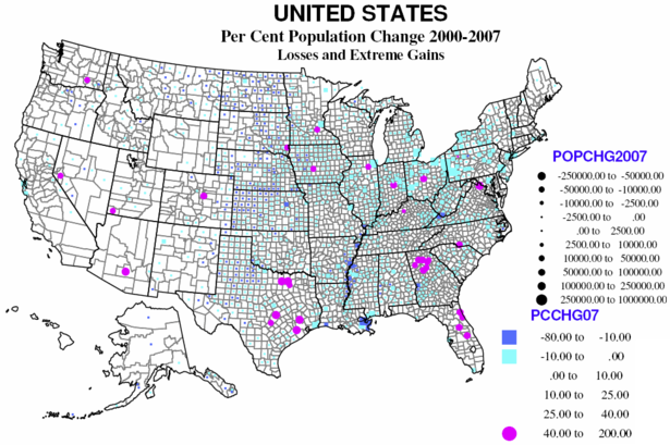
    The largest contiguous area of counties with losses remains the same as it was in the 1970s, 1980s and 1990s: the “high plains” from Mexico to Canada (actually continuing in Canada). Probably 90 percent of counties lost population, especially in Kansas, Nebraska and North Dakota, and extending into the Midwest agricultural heartland of Iowa, northern Missouri, southern Minnesota and western Illinois.

    Other traditional areas of losses which continue from the 1970s through 1990s include the coal counties of Appalachia (Kentucky, West Virginia), and the “Black Belt” from Arkansas and Louisiana through the Mississippi Delta and on through parts of Alabama, Georgia, South and North Carolina into Virginia.

    Again repeating past patterns are losses in some of the large core counties of Megalopolis, as Philadelphia and Baltimore, and elsewhere (St. Louis, Chicago, Minneapolis and even San Francisco). The highest rates of loss were again in and around New Orleans, small counties in Mississippi and Nevada, and Montana, North and South Dakota.

    The 33 rapidly growing counties are ALL suburban except for the new metropolitan area of St. George, Utah. Suburban Atlanta dominates, followed by northeastern Florida, and selected suburbs of Columbus, OH, Indianapolis, Charlotte, Chicago, Minneapolis, Washington, DC, Des Moines, Denver, Reno, Houston, Dallas, and Austin. The largest absolute gains (many areas are now hurting economically) were Maricopa (Phoenix), Harris (Houston), Riverside and San Bernardino, Clark (Las Vegas), Los Angeles, and suburbs of Dallas and San Antonio.

    Migration

    Immigration dominates the news, but there is also emigration, and the difference between these is ‘net’ international migration. Data on immigration and emigration are not very certain or reliable, as people leaving don’t have to tell anyone, and many entering are equally reticent. Yet there is a clear pattern from the map of the 416 counties. Overall the areas of net loss tend to be the same as for losses in overall population.

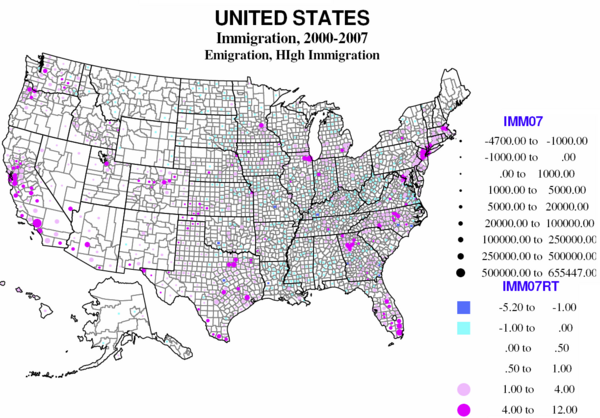
    Counties where immigrants greatly exceed emigrants are both the core counties of the largest metropolitan areas and their largest suburban counties, but especially in the west, Texas, Florida, and the Atlantic coast metropolitan cores from Atlanta to Boston, California, Texas, Florida, and metropolitan New York city. Mexican immigration is the largest, but there is significant immigration from the rest of Latin America, from Asia and from Eastern Europe. Most of the immigrant destinations are metropolitan, but include some rural small town areas, typically with food processing, an industry dependent on low wage immigrants (TX, AR, OK, KS, NE, IA).

    Largest absolute gains are to Los Angeles, Cook, New York City, Miami, Houston, Dallas, Orange County, Phoenix and Santa Clara, with a bias to the southwest, Florida and New York City. The highest immigration rates are in part the same, Miami, Queens, Hudson NJ, Santa Clara, but high rates also characterize Washington DC suburbs, two Kansas counties (food processing), and a Colorado county (workers for ski resorts).

    Significant numbers of non-immigrants also move, and as many as a third probably crossed county lines since 2000. In much of America the balance between in and out migration is close, but for many regions, “net” migration is the most important component of change.

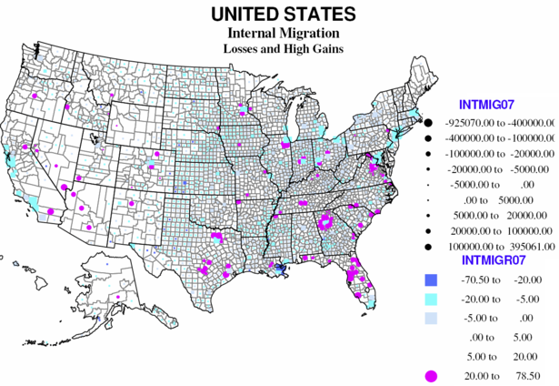
    Overall two thirds of American counties reported a net loss from internal migration, 29 at a level more than 20 percent of the base population. Only 118 have high rates of net in-migration (over 20 percent). Large absolute losses characterize most large metropolitan core counties, including coastal California, Dallas, Miami, New Orleans, megalopolis core counties (from Maryland to Massachusetts), and the Great Lakes and Midwest. Smaller absolute net out-migration prevails over most rural small-town America, especially the Great Plains, and agricultural Midwest and Great Lakes, the Black Belt across the south, and includes much of the southwest.

    Internal domestic migration represents a distinctive geography. In the west many were inland smaller metropolises, as well as many rural small town environmentally attractive counties that received many of the out-migrants from the large coastal metropolises. In the Midwest and northeast gains were strongly suburban (often local flows from the core counties). In the south rapid gains continued to dominate much of Florida, and metropolitan suburbs, especially around Washington DC, Atlanta, Dallas, and Austin-San Antonio, fueled both by continuing in-region rural to urban flows and by migration from the north to the south.

    The losses include the usual suspects, the core counties of the largest metro areas, including Dallas, Miami, and Orange counties, with the native-born displaced to the suburbs and beyond. The largest absolute gains include some central counties, like Maricopa and Clark (but which are also themselves suburban), major suburban counties of Los Angeles, Dallas, Houston, Phoenix, Chicago, and a newcomer, Wake county NC (Raleigh). The highest rates of net in-migration are mostly suburban, Atlanta, Dallas, Washington DC, Denver, Chicago, but also a few smaller counties, as in Pennsylvania and South Dakota.

    The Role of Natural Increase

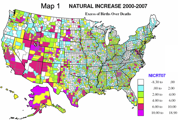
    One of the indicators of diversity in America is the remarkable variation in the role of natural increase (or decrease) – that is the difference between births and deaths in an area – in the story of population change.

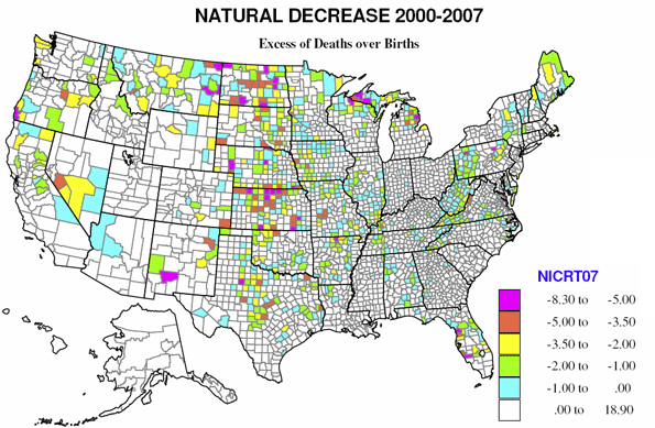
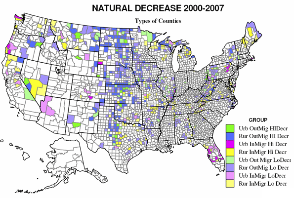
    Almost 30 percent of US counties experience natural decrease, and only a little over 10 percent (337) have high rates of natural increase (6% or more growth in 7 years). Natural decrease is mainly a function of age structure, where the young of child-raising age have left, OR where unusual numbers of the elderly have moved in, dominating the population.

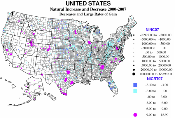
    There are four distinct regions of natural decrease. The largest, absolutely and relatively, is Appalachia, from extreme northern Georgia, through smaller parts of Tennessee and North Carolina, western Virginia, most of West Virginia, and both the greater Pittsburgh and the Scranton-Wilkes Barre region of northeastern Pennsylvania. Much is a historic region of coal (and steel) production, and often poor transport links to the rest of country. The region has suffered loss of the young, often for 40 years or more.

    The second large region of natural decrease is entirely different in character, namely mid-Florida, centered on Tampa-St, Petersburg and Sarasota, as a result of the aging in place of massive numbers of retirees from the north moving to Florida over the last 50 years.

    The third region is much more extensive, covering most of the Great Plains and rural Midwest, from Texas and Arkansas to the Dakotas, Minnesota and Montana, regions again suffering long-term loss of the young population to greater opportunities in the city.

    The last smaller region is the Michigan-Wisconsin upper peninsula, where losses can be traced to the result of declining mining and forestry. Counties in New Mexico, Arizona, and northern California are somewhat like Florida with large numbers of retirees, while those in coastal Oregon and Washington are in part like upper Michigan, but with many retirees as well.

    The 112 counties where births greatly exceed deaths, not surprisingly, reflect a very different geography. They do represent, as is often pointed out, a shift to metropolitan areas but importantly not to the core cities but the suburban hinterlands. Most prominent areas of high natural increase are primarily suburban areas around metropolitan Houston, Dallas, San Antonio, Atlanta, Washington DC, Chicago, Minneapolis and Raleigh, NC. Many of these areas are also affected by in-migration of Hispanic families.

    The other reason for high natural increase is higher fertility – families with above replacement numbers of children, often for reasons of religion or ethnicity, and also reinforced by in-migration of young adults. On the map, Native American Indian reservations stand out, as in North and South Dakota, Wisconsin, Montana, and Alaska, although these numbers are still slow. Mormon Utah and Idaho demonstrate high fertility, family size and shares of births, in rural as well as urban counties. But the dominant area of high natural increase is clearly the extensive southwestern region of Mexican heritage and in-migration over recent decades, in Texas, California, Colorado, New Mexico, Arizona, and eastern Washington, plus selected counties in the high plains, e.g., Kansas and Oklahoma. The final bastions for young families and higher natural increase are military dominated counties, as in Georgia, North Carolina and Kansas.

    In absolute losses, parts of Florida and Pennsylvania and the northern Great Plains stand out. Relative gains are highest in Hispanic, Native American Indian and Mormon counties. These are impressive numbers – the surplus of births over deaths as a share of the total population.

    Why the Differences?

    What makes counties lose or gain people? The US has a diverse and restless population. Counties vary greatly in attractiveness to immigrants from abroad or migrants from other states, broadly because of real or perceived “opportunities,” characteristics of jobs or amenities which may lure migrants from less competitive or attractive areas.

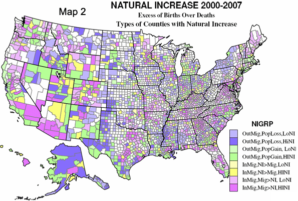
    The map divides the counties into nine sets, based on the relative importance of natural increase or decrease, emigration and immigration and in-migration and out-migration. The 1439 counties which lost population include 165 for which the main reason for loss is from natural decrease; of these one subgroup lost overall despite net immigration, the other’s loss was aggravated by net out-migration as well. The larger set of counties with population losses, 1184, are those for which the loss is mainly attributable to net out-migration, with two subgroups, one with loss despite natural increase, the other with loss magnified by natural decrease.

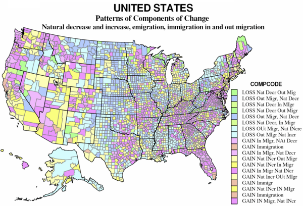
    On the map the “darker” green counties (89) had a large natural decrease and a smaller net out-migration; the “lighter” green (76) had natural decrease, exceeding a smaller net in-migration. These counties for which natural decrease dominates are scattered across the Great Plains from Texas to Canada, together with clusters from Appalachia (VA, WV, PA, and NY), northern MI-WI, and a few declining natural resource areas in the west.

    The “darker” blue counties (486) are dominated by net out-migration, but also had natural decrease. The “lighter” blue counties (698) had natural increases but these were much exceeded by net out-migration. These counties are often interspersed with the “green” counties, dominated by natural decrease. These 1184 counties – over one-third of counties and of US territory – constitute a large swath of the Plains and Midwest, large parts of New York and Pennsylvania, the coal counties of Kentucky and West Virginia, and the “Black Belt” across the south from Louisiana and Arkansas to southern Virginia. Finally they include sparsely populated resource counties in Alaska and parts of the west. Overall, the counties losing population tend to be non-metropolitan and interior, except for the declining industrial metropolitan counties of the “Rust Belt”.

    Gainers

    The gaining counties consist of three broad groups — 755 for which natural increase is the main contributor to growth, with subsets of 420 growing despite net out-migration, and 335 with net in-migration as well. The second consists of 104 counties for which immigration is the predominant basis for growth. Finally there are 933 counties for which net in-migration is the main contributor to growth, with subsets with natural decrease with natural increase.

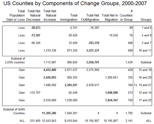
    The “yellow” counties (755) gained population mainly because of natural increase; the light yellow counties (420) grew despite often substantial net out-migration; the darker yellow counties (335) also had a smaller net in-migration, and are thus among the more ”successful” more rapidly growing US counties. The former are especially prevalent in cities of the west – e.g. Los Angeles, San Diego, Houston, Dallas – with sizable immigrant populations (see the table) and higher fertility and displacement of the native-born, but yellow counties are also common in non-metropolitan and small metropolitan and suburban areas of the Great Lakes states, the outer Megalopolis, and urban industrializing parts of the south. The “dark” yellow areas are in the same regions, and are very often the areas gaining migrants from the “light” yellow areas, as can be seen in California, Arizona, Utah, Washington and Colorado.

    The “orange” counties, only 104, are those where immigration is the main source of growth. These are somewhat scattered, but especially common in New England and Middle Atlantic states, selected counties of the Plains (often with food processing plant growth) and northern Pacific Coast metropolitan regions, as the San Francisco bay region, Portland and Seattle.

    The “magenta” counties (933) are those for which net in-migration dominates growth. The lighter magenta for those with natural decrease (213), the darker magenta for those with natural increase as well. All these tend to be the most rapidly growing counties in the country, and tend to occur together. The main difference with counties with natural decrease are those with an older age structure, but which are nevertheless attractive to in-migrants. From the map these occur in two main settings: traditional areas of amenity migration, most obviously covering much of Florida, but also widespread in northern New England, northern Michigan, Wisconsin and Minnesota, the Ozarks, parts of the Tennessee valley, and across much of the west, with particular swaths in western Montana, coastal Oregon and Washington and northern California. The second setting is the exurban environs of major metropolitan areas, where new growth is invading formerly rural areas.

    The final, largest set of counties with natural increase as well as high in-migration (720 counties), are the stereotypical winners in the contemporary “growth races” – based on a combination of employment growth and metropolitan or environmental amenities. These tend especially to be southern and western metropolitan areas, small as well as large. The most dominant regions are greater Washington DC, greater Atlanta, Dallas and Houston, Portland, Denver, Phoenix, most of Florida, and – perhaps surprisingly – substantial parts of the north-south borderlands, including Tennessee, Kentucky, Arkansas, Oklahoma, and Missouri.

    What about the recession? It’s hard to judge the relative effects of the current severe recession on likely near- or longer-term growth. Clearly, the collapse of housing markets are slowing the growth of such rapidly growing places as Phoenix and Las Vegas, but this does not mean they won’t regain their general attractiveness and economic viability. The particularly severe job losses in the already hurting western Rust Belt will likely aggravate the recent pattern of decline which predated the recession and could get much worse.

    Richard Morrill is Professor Emeritus of Geography and Environmental Studies, University of Washington. His research interests include: political geography (voting behavior, redistricting, local governance), population/demography/settlement/migration, urban geography and planning, urban transportation (i.e., old fashioned generalist)