Author: Wendell Cox

Highest Cost Rental Markets: Even Worse for Buyers

There is considerable concern about rising rents, especially in the most expensive US housing markets. Yet as tough as rising rents are, the high rent markets are also plagued by even higher house costs relative to the rest of the nation. As a result, progressing from renting to buying is all the more difficult in these areas.

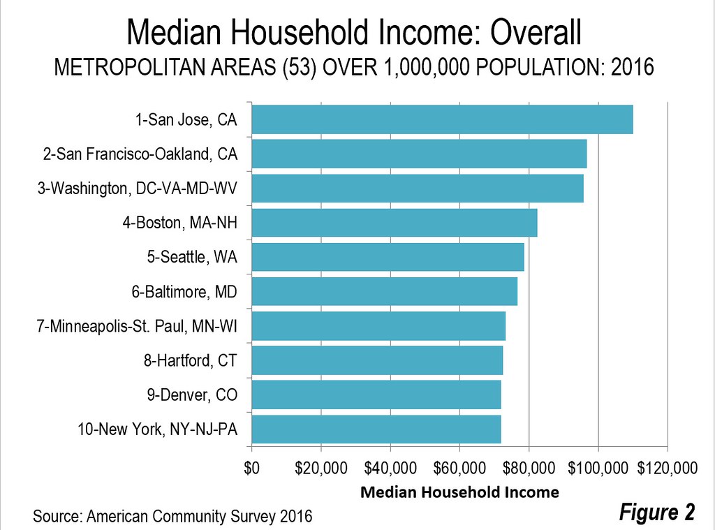
This is illustrated by American Community Survey data for the nation’s 53 major housing markets (metropolitan areas with more than 1,000,000 residents). The range in median contract rent between the major housing markets 3.1 times, with San Jose being the most expensive and Rochester the least. The range in median house values was more than double that, at 6.6 times, between highest cost San Jose and lowest cost Pittsburgh. Thus, house prices in the most expensive markets tend to be far higher in relation to rents than in the less expensive markets.

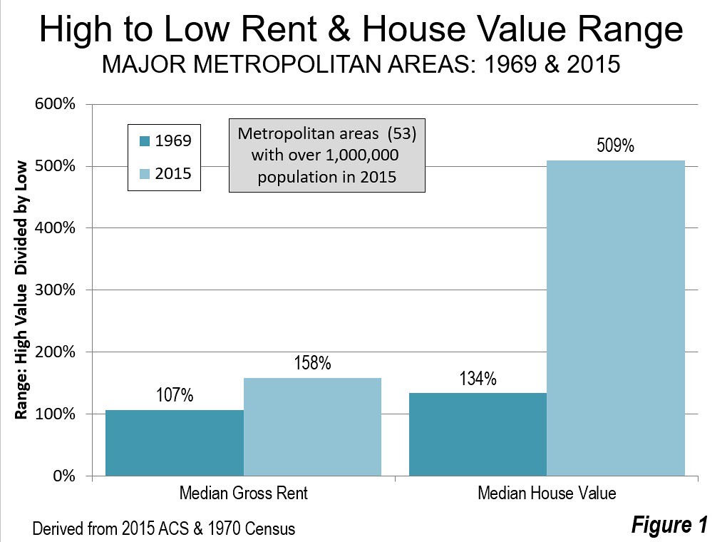
The rising difference between house values and rents was noted last year in The House Prices are Too Damned High, which showed that from 1969 to 2015, the difference in the range between rentals and house values rose from 51 percentage points to 375 percentage points (Figure 1). It is no coincidence that 1969 was the last census data before far more strict land use regulations were implemented in some major housing markets.

The House Value-to-Rent Ratio

This is illustrated by the median house value-to-rent ratio, which is calculated by dividing the median house value by the median contract rent per year (monthly times 12). Overall in 2016, the median contract rent was $841 in the United States, while the median house value was $205,000. This calculates to a value-to-rent ratio of 20.3.

Where Housing Aspiration is Most Challenging

California, long home to house prices far above the rest of the nation dominates the list of housing markets in which it is hardest for buyers to move up to home ownership. The worst market is the San Francisco metropolitan area, where the median house value in 2016 was nearly 40 times the median annual rent (39.6) and nearly twice the national figure of 20.3. San Jose is the second worst market, with a value-to-rent ratio of 38.7. Los Angeles is third where the median house value is 36.9 times the median annual rent. There is a larger gap down to San Diego, ranked fourth worst, where there is a median value-to-rent ratio of 31.1. Sacramento is also in the least friendly five for renters aspiring to be buyers, with a value-to-rent ratio of 29.6. This may be a surprising finding and is discussed further below. California’s other major market, Riverside-San Bernardino does better, ranking 13th worst, with a value-to-rent ratio of 24.5.

Even with New York’s notoriously high rents, it did not muscle out California in the worst five. New York’s s value-to-rent ratio was 29.5 The balance of the 10 markets in which moving from renting to buying is most difficult also includes #7 Boston (28.1), #8 Portland (27.9), #9 Providence (27.7) and #10 Seattle (27.2).

Comparison with Demographia Housing Affordability Ratings

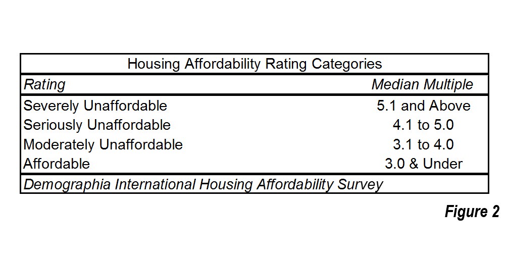
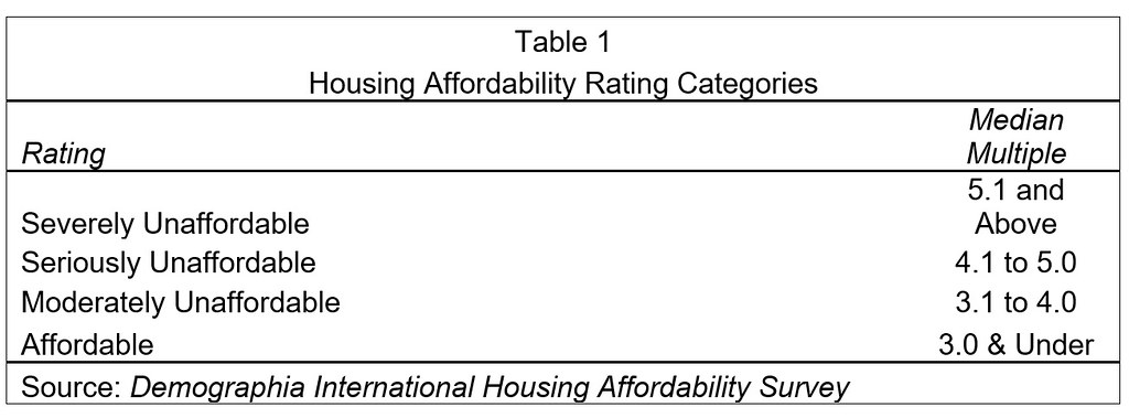
The eleven housing markets with the highest value-to-rent ratios have ratings of “severely unaffordable” in the 13th Annual Demographia International Housing Affordability Survey. This is the least affordable rating (Figure 2) and indicates a median multiple of 5.1 or higher (median house price divided by median household income). The 12th highest value-to-rent ratio is in Salt Lake City, which is rated “seriously unaffordable,” the second most unaffordable category. Thirteenth ranked Riverside-San Bernardino was the only other severely unaffordable major U.S. housing market in the Demographia survey.

Each of the severely unaffordable markets have land use restrictions that make it virtually impossible to build the low-cost suburban tract housing crucial to retaining housing affordability. In such markets, Buildzoon.coms’ economist Issi Romem has shown that house values have become detached from construction costs, largely the result of rising land prices (which are associated with stronger land use regulation, especially urban containment policy).

The Surprising Case of Sacramento

Sacramento’s high cost housing may come as a surprise. Sacramento has often “slipped under the radar” as a severely unaffordable market, yet was so from 2004 through 2008.Sacramento had reached a median multiple of 6.8 in 2005 before the housing bust and was less affordable than Vancouver, the third least affordable housing market out of nine nations rated in 2016 by Demographia. Sacramento again became severely unaffordable in last year’s Demographia survey reaching a median multiple of 5.1. But there is reason for concern in Sacramento, which has seen its median multiple rise from 2.9 to 5.1 in just four years. Any continuation of such this trend could result in a material deterioration of Sacramento’s value-to-rent ratio, made all the more likely by California’s overly restricted housing and land use regulations.

The Value-to-Rent Ratio and Inequality

Rising inequality is a widespread concern. Yet, as researchers have shown, much of the expanding inequality is centered in the value of owned housing, which has been associated with more restrictive land and housing regulation. In the United States, the price is being paid for by younger households, who are faced with greater student loan debts and a less lucrative economy. It is also paid for by ethnic minority households, whose more limited incomes are making the jump to home ownership even more difficult (See: Progressive Cities: Home of the Worst Housing Inequality).

Median House Value to Median Contract Rent Ratios
53 Major US Housing Markets (Metropolitan Areas)
Worst Markets for Moving from Renting to Buying
Rank	Housing Market (Metropolitan Area)	Value-to-Rent Ratio	Median Contract Rent (Monthly)	Median House Value	Housing Affordabilty Rating
1	San Francisco-Oakland, CA	39.56	$1,677	$796,100	Severely Unaffordable
2	San Jose, CA	38.69	$1,964	$911,900	Severely Unaffordable
3	Los Angeles, CA	36.92	$1,305	$578,200	Severely Unaffordable
4	San Diego, CA	31.07	$1,415	$527,600	Severely Unaffordable
5	Sacramento, CA	29.62	$1,022	$363,300	Severely Unaffordable
6	New York, NY-NJ-PA	29.05	$1,223	$426,300	Severely Unaffordable
7	Boston, MA-NH	28.14	$1,222	$412,700	Severely Unaffordable
8	Portland, OR-WA	27.89	$1,031	$345,000	Severely Unaffordable
9	Providence, RI-MA	27.77	$796	$265,300	Seriously Unaffordable
10	Seattle, WA	27.23	$1,198	$391,500	Severely Unaffordable
11	Denver, CO	24.79	$1,174	$349,200	Severely Unaffordable
12	Salt Lake City, UT	24.60	$907	$267,800	Moderately Unaffordable
13	Riverside-San Bernardino, CA	24.47	$1,086	$318,900	Severely Unaffordable
14	Washington, DC-VA-MD-WV	23.74	$1,444	$411,400	Seriously Unaffordable
15	Baltimore, MD	23.21	$1,055	$293,900	Moderately Unaffordable
16	Milwaukee,WI	23.07	$737	$204,000	Seriously Unaffordable
17	Hartford, CT	22.83	$903	$247,400	Moderately Unaffordable
18	Raleigh, NC	22.56	$878	$237,700	Moderately Unaffordable
19	Philadelphia, PA-NJ-DE-MD	22.27	$919	$245,600	Moderately Unaffordable
20	Las Vegas, NV	22.06	$883	$233,700	Seriously Unaffordable
21	Phoenix, AZ	21.97	$876	$231,000	Seriously Unaffordable
22	Richmond, VA	21.81	$868	$227,200	Moderately Unaffordable
23	Minneapolis-St. Paul, MN-WI	21.64	$926	$240,500	Moderately Unaffordable
24	Virginia Beach-Norfolk, VA-NC	21.27	$940	$239,900	Moderately Unaffordable
25	Austin, TX	21.20	$1,035	$263,300	Seriously Unaffordable
26	Cincinnati, OH-KY-IN	21.08	$653	$165,200	Affordable
27	Nashville, TN	21.00	$829	$208,900	Moderately Unaffordable
28	Louisville, KY-IN	20.94	$645	$162,100	Moderately Unaffordable
29	St. Louis,, MO-IL	20.64	$683	$169,200	Affordable
30	Chicago, IL-IN-WI	20.60	$930	$229,900	Moderately Unaffordable
31	Kansas City, MO-KS	20.38	$711	$173,900	Affordable
32	Columbus, OH	20.15	$712	$172,200	Affordable
33	Birmingham, AL	20.15	$637	$154,000	Moderately Unaffordable
34	New Orleans. LA	19.89	$788	$188,100	Moderately Unaffordable
35	Oklahoma City, OK	19.86	$647	$154,200	Affordable
36	Tucson, AZ	19.82	$716	$170,300	Moderately Unaffordable
37	Charlotte, NC-SC	19.77	$793	$188,100	Moderately Unaffordable
38	Pittsburgh, PA	19.62	$631	$148,600	Affordable
39	Miami, FL	19.36	$1,122	$260,600	Severely Unaffordable
40	Grand Rapids, MI	19.20	$714	$164,500	Affordable
41	Atlanta, GA	18.72	$880	$197,700	Moderately Unaffordable
42	Buffalo, NY	18.63	$636	$142,200	Affordable
43	Cleveland, OH	18.47	$659	$146,100	Affordable
44	Indianapolis. IN	18.43	$694	$153,500	Affordable
45	Detroit, MI	18.37	$729	$160,700	Affordable
46	Jacksonville, FL	18.33	$853	$187,600	Moderately Unaffordable
47	Dallas-Fort Worth, TX	18.13	$869	$189,100	Moderately Unaffordable
48	Orlando, FL	17.72	$948	$201,600	Seriously Unaffordable
49	Memphis, TN-MS-AR	17.69	$671	$142,400	Moderately Unaffordable
50	Houston, TX	17.36	$871	$181,400	Moderately Unaffordable
51	San Antonio, TX	16.65	$802	$160,200	Moderately Unaffordable
52	Tampa-St. Petersburg, FL	16.61	$879	$175,200	Seriously Unaffordable
53	Rochester, NY	15.97	$725	$138,900	Affordable

Sources: American Community Survey 2016, 13th Annual Demographia International Housing Affordability Survey.

Wendell Cox is principal of Demographia, an international public policy and demographics firm. He is a Senior Fellow of the Center for Opportunity Urbanism (US), Senior Fellow for Housing Affordability and Municipal Policy for the Frontier Centre for Public Policy (Canada), and a member of the Board of Advisors of the Center for Demographics and Policy at Chapman University (California). He is co-author of the “Demographia International Housing Affordability Survey” and author of “Demographia World Urban Areas” and “War on the Dream: How Anti-Sprawl Policy Threatens the Quality of Life.” He was appointed to three terms on the Los Angeles County Transportation Commission, where he served with the leading city and county leadership as the only non-elected member. He served as a visiting professor at the Conservatoire National des Arts et Metiers, a national university in Paris.

Photograph: Sacramento – One of 5 most difficult markets for moving from renting to buying.

October 27, 2017

Housing Unaffordability Policies: “Paying for Dirt”

Issi Romem, buildzoom.com’s chief economist has made a valuable contribution to the growing literature on the severe unaffordability of housing in a number of US metropolitan areas. The disparities between the severely unaffordable metropolitan areas (read San Jose, San Francisco, Los Angeles, San Diego, Portland, Seattle, Portland, Denver, Miami, New York, Boston, Sacramento and Riverside-San Bernardino) and the many more affordable areas in America are described in “Paying For Dirt: Where Have Home Values Detached From Construction Costs“. Romem points out that: “In the expensive U.S. coastal metros, home prices have detached from construction costs and can be almost four times as high as the cost of rebuilding existing structures.”

“Paying for dirt” refers to the ballooning land costs that now comprise an unprecedented part of house values, such as in the severely unaffordable metropolitan markets above. This has created an environment where affordability is impossible. In many of these metropolitan areas, a modest house commands an exorbitant price well beyond the financial capacity of most middle income households. Land has become so expensive that it doesn’t matter what is built on it, whether the average house or a tent, the price will be too high. The market distortions are so great that Romem is able to show that, for example, the average house value in Columbus, Ohio, a delightful metropolitan area, is less than the average land value per lot in Portland (Oregon).

The research suggests that the variation in construction costs between US metropolitan areas pales by comparison to the differences in the land costs. In the most expensive housing market, San Jose, the average house value is seven times that of Buffalo, the least expensive. By contrast, the highest cost construction market (San Francisco) is only twice as expensive as the least (Las Vegas). The land cost differences are stark, exceeding a 40 times difference in San Jose compared to Buffalo or Indianapolis. In Indianapolis, new detached house construction in 2017 was 2.5 times that of much larger and more expensive San Diego.

The Research

Romem’s research is similar to that of Harvard’s Edward Glaeser and Wharton’s Joseph Gyourko (“The Economic Implications of Housing Supply”), who separated US metropolitan areas into those with “well-functioning” housing markets and those without. In the well-functioning housing markets homebuilders could construct houses for what the researchers called the “minimum profitable production cost. Their list of high cost markets that are not well-functioning nearly matches Romem’s list of metropolitan areas where land costs have risen most compared to construction costs. Romem provides estimates down to the ZIP Code level in major metropolitan areas, illustrating a substantial depth of analysis.

Consistent with Glaeser and Gyourko, Romem finds that “absent restrictions on housing supply, competition among developers tends to maintain average metropolitan home prices tethered to the cost of construction.”

The Problem of Excessive Land Use Regulations

In the highly regulated metropolitan areas, promoters of the urban containment policies often hide behind the fiction of topographical or geographical barriers as having created the land scarcity. A particular favorite for this blather is the San Francisco Bay Area (which includes the San Francisco and San Jose metropolitan areas) that has driven house prices up so much. There is no question that topography and geography can create such a shortage, as this photograph of Maldives capital Male shows. But nothing in the Bay Area looks like Male (photograph above).

But San Francisco and San Jose are nothing like Male. In fact, the San Francisco Bay Area has enough land for development that millions of new houses could be constructed. San Francisco’s urbanization is dense, with at least 15 more residents per square mile than the New York urban area (population centre). Its population, nearly one-third that of New York, lives in an even smaller one-fourth the land area. There would be no need for urban containment in the Bay Area if the topography genuinely limited development.

Toward A More Unequal Society

In a note, Romem says that “The stark differences in land value per home are driven largely by land use policy enacted in the expensive coastal metros since the 1970s, which has inhibited these cities’ growth. These metro areas have gradually slowed down their outward expansion, i.e. they have had success in stemming sprawl, but they have failed to compensate through densification. As a result, the economic vitality of these metros has been channeled away from population growth and into housing price growth.”

“Stemming sprawl” while maintaining housing affordability through higher densities is a time-worn theory. The record seems to indicate that it is more likely Santa will come down the chimney than density will solve the problem. There are no virtually examples of housing markets (metropolitan areas) where increasing densities has restored affordability. This is not to suggest there is no value to increased density, but rather that it is an all too convenient diversion from solutions that have a chance of working.

Appropriately, Romem puts this childish notion to rest that increasing densities “will reduce the land value component of homes simply by dividing a fixed land value over a greater number of units.”

The bottom line is that the house price appreciation in the high cost metropolitan areas suppresses population by “selectively determining who can and cannot afford to live there” according to Romem. This policy outcome could not be more inconsistent with encouraging economic aspiration among middle-income households, who pay the price of the greater inequality imposed by public policy. Further, those effectively “zoned out” by these policies have greater financial challenges than their parents, who generally grew up in periods of greater economic growth and were not saddled with unprecedented student loan debt.

The financial and exclusionary challenges weigh particularly hard on the large number of disadvantaged African-Americans and Hispanics, especially those living in the most progressive cities, where pious pronouncements about affordable housing initiatives are boilerplate, but rarely amount to anything remotely substantive. In fact, distorted land and housing markets in the expensive metropolitan areas represent a colossal government failure.

Necessary Reforms

To the contrary, housing affordability requires well-functioning housing markets. It requires home values that have not become detached from construction costs. A minimum condition is that land use regulations not stand in the way of building low cost housing tracts on the periphery of urban areas. This does not require building on the monstrous size lots of suburban Boston, where zoning and other land use restrictions have made housing far more expensive and exclusive than it needs to be. The key is to restore the competitive market for land, so that houses on comparatively small lots, such as one-quarter or one-fifth of an acre can be built at the historic land costs (including necessary infrastructure). Glaeser and Gyourko found this factor to account for about 20 percent of final purchase prices (as did I).

Romem expresses a hope that things will improve. “The disparity between the appearance of homes and their price tags is more than a home buyer’s gripe: it is a telltale indication of restricted housing supply. Such restrictions – rules governing land use, installed by incumbent residents or their predecessors – are exclusionary by nature and amount to the gating of access to opportunity. Hopefully, this study has helped identify where gates must be opened.”

Indeed.

Wendell Cox is principal of Demographia, an international public policy and demographics firm. He is a Senior Fellow of the Center for Opportunity Urbanism (US), Senior Fellow for Housing Affordability and Municipal Policy for the Frontier Centre for Public Policy (Canada), and a member of the Board of Advisors of the Center for Demographics and Policy at Chapman University (California). He is co-author of the “Demographia International Housing Affordability Survey” and author of “Demographia World Urban Areas” and “War on the Dream: How Anti-Sprawl Policy Threatens the Quality of Life.” He was appointed to three terms on the Los Angeles County Transportation Commission, where he served with the leading city and county leadership as the only non-elected member. He served as a visiting professor at the Conservatoire National des Arts et Metiers, a national university in Paris.

Photograph: Male (capital of the Maldives): Where there are genuine topographical constraints.
https://upload.wikimedia.org/wikipedia/commons/6/67/Male_maldives.jpg

October 21, 2017
San Francisco’s Abundant Developable Land Supply

The San Francisco Bay Area (home of the San Francisco and San Jose metropolitan areas), which has often been cited as a place where natural barriers have left little land for development. This is an impression easily obtained observing the fairly narrow strips of urbanization on both sides of San Francisco Bay, hemmed in by hills.

However the Bay Area’s urbanization long ago leapt over the most important water bodies and then the Berkeley Hills to the east. Not only is the San Francisco Bay Area CSA high density, but it is also spatially small. In 2016, the San Francisco built-up urban area was only the 23rd largest in land area in the world. New York, the world’s largest built-up urban area in geographical expanse is more than four times as large.

There is plenty of developable land in the San Francisco Bay Area. Data in a 1997 state analysis indicated that another 1,500 to 4,300 square miles (3,900 to 11,000 square kilometers) could be developed in the Bay Area CSA. The lower bound assumed no farmland conversion and stringent environmental regulation. The report also found that in recent years, residential development had become marginally denser, yet not incompatible with the detached housing remains the preference in California (Figure). The state has more than enough developable land for future housing needs.

Demographia International Housing Affordability Survey with a median multiple of 9.6 (median house price divided by median household income) and the San Francisco metropolitan area is 7th worst, with a median multiple of 9.2. Before the evolution toward urban containment policies began, the median multiples in these metropolitan areas (and virtually all in the United States) were around 3.0 or less.

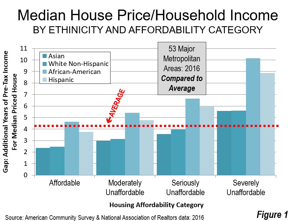
The decades old Bay Area housing affordability crisis, and that of other urban containment metropolitan areas that are now seriously unaffordable (median multiples over 5.0) seeking to force higher densities, is more the result of policy than nature.

Note on Method: Some of the CSA urban population is not in the continuous urbanization of San Francisco-San Jose built-up urban area, such as in the Santa Rosa, Stockton and Santa Cruz urban areas. This analysis is based on data from the California Department of Housing and Community Development and the U.S. Census Bureau. It is based on an estimate of additional development occurring from 1996 to 2010 and the land remaining after deduction of recently developed land. The population capacity assumes the “marginally higher” densities used by the California Department of Housing and Community Development, which it notes would not require substantial changes in the “current form of housing development” (1997).

October 20, 2017

Progressive Cities: Home of the Worst Housing Inequality

America’s most highly regulated housing markets are also reliably the most progressive in their political attitudes. Yet in terms of gaining an opportunity to own a house, the price impacts of the tough regulation mean profound inequality for the most disadvantaged large ethnicities, African-Americans and Hispanics.

Based on the housing affordability categories used in the Demographia International Housing Affordability Survey for 2016 (Table 1), housing inequality by ethnicity is the worst among the metropolitan areas rated “severely unaffordable.” In these 11 major metropolitan area markets, the most highly regulated, median multiples (median house price divided by median household income) exceed 5.0. For African-Americans, the median priced house is 10.2 times median incomes. This is 3.7 more years of additional income than the overall average in these severely unaffordable markets, where median house prices are 6.5 times median household incomes. It is only marginally better for Hispanics, with the median price house at 8.9 times median household incomes, 2.4 years more than the average in these markets (Figure 1).

The comparisons with the 13 affordable markets (median multiples of 3.0 and less) is even more stark. For African-American households things are much better than in the more progressive and most expensive metropolitan areas. The median house prices is equal to 4.6 years of median income, 5.5 years less than in the severely affordable markets. Moreover, for African-Americans, housing affordability is only marginally worse than the national average in the affordable market.

Things are even better for Hispanics, who would find the median house price 3.8 times median incomes, 5.1 years less than in the severely affordable markets. This is better than the national average housing affordability.

Among the four markets rated “seriously unaffordable,” (median multiple from 4.1 to 5.0) the inequality is slightly less, with African-Americans finding median house prices equal to 2.2 years of additional income compared to average. The disadvantage for Hispanics is 1.5 years.

In contrast, inequality is significantly reduced in the less costly “moderately unaffordable” markets (median multiple of 3.1 to 4.0) and the “affordable” markets (median multiple of 3.0 and less).

The discussion below describes the 10 largest and smallest housing affordability gaps for African-American and Hispanic households relative to the average household, within the particular metropolitan markets. The gaps within ethnicities compared to the affordable markets would be even more. The four charts all have the same scale (a top housing affordability gap of 10 years) for easy comparison.

able 2 illustrates housing affordability gaps by major metropolitan areas. There are also housing affordability ranking gap tables by African-American households (Table 3) and Hispanic households (Table 4).

Largest Housing Affordability Gaps: African American

African-Americans have the largest housing affordability inequality gap. And these gaps are most evident in some of the nation’s most progressive cities. The largest gap is in San Francisco, where the median income African-American household faces median house prices that are 9.3 years of income more than the average. In nearby San Jose ranks the second worst, where the gap is 6.2 years. Overall, the San Francisco Bay Area suffers by far the area of least housing affordability for African-Americans compared to the average household.

Portland, long the darling of the international urban planning community, ranks third worst, where the median income African-American household to purchase the median priced house. Milwaukee and Minneapolis – St. Paul ranked fourth and fifth worst followed by Boston, Seattle, Los Angeles, Sacramento and Chicago (Figure 2).

Largest Housing Affordability Gaps: Hispanics

Two of the three worst positions are occupied by the two metropolitan areas in the San Francisco Bay Area. The worst housing affordability gap for Hispanics is in San Jose, a more than one-quarter Hispanic metropolitan area where the median income Hispanic household would require 5.0 years of additional income to pay for the median priced house compared to the average. Boston ranks second worst at 3.9. San Francisco third worst at 3.3 years. Providence and New York rank fourth and fifth worst. The second five worst housing inequality for Hispanics is in San Diego, Hartford, Rochester, Philadelphia and Raleigh (Figure 3).

The San Francisco Bay Area: “Inequality City”

Perhaps no part of the country is more renowned for its progressive politics and politicians than the San Francisco Bay Area. Yet, in housing equality, the Bay Area is anything but progressive. If the African-American and Hispanic housing inequality measures are averaged, disadvantaged minorities face house prices that average approximately 6.25 years more years of median income in San Francisco and 5.60 more years of median income in San Jose.

Moreover, no one should imagine that recent state law authorizing a $4 billion “affordable housing” bond election will have any significant impact. According to the Sacramento Bee, voter approval would lead to 70,000 new housing units annually, when the need for low and very low income households is 1.5 million. The bond issue would do virtually nothing for the many middle-income households who are struggling to pay the insanely high housing costs California’s regulatory nightmare has developed.

Smallest Housing Affordability Gaps: African-American

Tucson has the smallest housing affordability gap for African-Americans. In Tucson, the median income African-American household would pay approximately 0.4 years (four months) more in income for the median priced house than the average household. In San Antonio, Atlanta and Tampa – St. Petersburg, the housing affordability gaps are under 1.0. Houston, Riverside – San Bernardino, Virginia Beach – Norfolk, Memphis, Dallas – Fort Worth and Birmingham round out the second five. It may be surprising that eight of the metropolitan areas with the smallest housing affordability gaps for African-Americans are in the South and perhaps most surprisingly of all that one of the best, at number 10, is Birmingham. (Figure 4).

Smallest Housing Affordability Gaps: Hispanic

Among Hispanic households, the smallest housing affordability gap is in Pittsburgh, where the median priced house would require less than 10 days more in median income for a Hispanic household compared the overall average. In Jacksonville the housing affordability gap for Hispanics would be less than two months. In Baltimore, Birmingham, St. Louis and Cincinnati, the median house price is the equivalent of less than six months of median income for an Hispanic household. Detroit, Memphis, Virginia Beach – Norfolk and Cleveland round out the ten smallest housing affordability gaps for Hispanics (Figure 5).

Housing Affordability is the Best for Asians

Recent American Community Survey data indicated that Asians have median household incomes a quarter above those of White Non-– Hispanics. This advantage is also illustrated in the housing affordability data. Asians have better housing affordability than White Non-– Hispanics in 37 of the 53 major metropolitan areas (over 1 million population).

The Importance of Housing Opportunity

Housing opportunity is important. African-Americans and Hispanics already face challenges given their generally lower incomes. However, by no serious political philosophy, progressive or otherwise, should any ethnicity find themselves even further disadvantaged by political barriers, such as have been created by over-zealous land and housing regulators.

Table 2
Housing Affordability Gap by Ethnicity: 2016
53 Major Metropolitan Areas (Over 1,000,000 Population)
Median Multiple (Median house price divided by median household income)

MSA	Median Multiple: All Households	Median Multiple: African-American	African American Housing Affordability Gap in Years	Ranked Most to Least Equal: African-American	Median Multiple: Hispanic	Hispanic Housing Affordability Gap in Years	Ranked Most to Least Equal: Hispanic	Exhibit: Median Multiple: Asian	Exhibit: Median Multiple: White Non-Hispanic

Atlanta, GA	2.95	3.83	0.88	3	3.65	0.70	13	2.30	2.45
Austin, TX	4.00	5.69	1.69	19	5.04	1.04	24	3.23	3.52
Baltimore, MD	3.29	4.75	1.46	12	3.64	0.34	3	2.60	2.83
Birmingham, AL	3.57	4.99	1.42	10	3.96	0.39	4	2.95	3.02
Boston, MA-NH	5.11	8.69	3.58	47	9.02	3.90	52	4.67	4.62
Buffalo, NY	2.48	4.79	2.32	38	4.58	2.10	43	2.90	2.20
Charlotte, NC-SC	3.47	4.95	1.47	13	4.77	1.30	32	2.31	3.08
Chicago, IL-IN-WI	3.56	6.30	2.75	43	4.45	0.90	20	2.69	2.94
Cincinnati, OH-KY-IN	2.53	4.70	2.17	35	2.99	0.46	6	1.75	2.33
Cleveland, OH	2.54	4.50	1.96	27	3.17	0.63	10	1.49	2.16
Columbus, OH	2.91	4.78	1.87	24	4.10	1.19	30	2.50	2.68
Dallas-Fort Worth, TX	3.56	4.98	1.42	9	4.70	1.14	26	2.55	2.87
Denver, CO	5.34	7.64	2.29	37	7.40	2.05	42	5.33	4.76
Detroit, MI	4.01	6.71	2.70	41	4.53	0.52	7	2.56	3.48
Grand Rapids, MI	2.68	4.66	1.98	28	3.85	1.16	28	2.95	2.53
Hartford, CT	3.18	4.88	1.70	20	5.48	2.29	47	2.78	2.82
Houston, TX	3.52	4.57	1.05	5	4.68	1.15	27	2.54	2.65
Indianapolis. IN	2.82	4.89	2.07	31	4.45	1.63	38	2.48	2.50
Jacksonville, FL	3.71	5.15	1.43	11	3.88	0.16	2	3.32	3.38
Kansas City, MO-KS	2.95	4.96	2.00	30	3.97	1.02	23	2.64	2.68
Las Vegas, NV	4.37	6.36	1.98	29	5.19	0.82	16	3.63	3.85
Los Angeles, CA	7.69	11.15	3.46	45	9.74	2.05	41	6.68	6.03
Louisville, KY-IN	2.99	4.90	1.91	25	3.92	0.93	21	2.48	2.71
Memphis, TN-MS-AR	3.12	4.37	1.25	8	3.68	0.56	8	2.13	2.29
Miami, FL	5.94	7.58	1.64	17	6.64	0.70	12	4.39	4.68
Milwaukee,WI	3.93	7.88	3.95	49	5.79	1.86	40	2.78	3.33
Minneapolis-St. Paul, MN-WI	3.24	6.83	3.59	48	4.64	1.40	34	3.25	3.01
Nashville, TN	3.74	5.43	1.69	18	5.04	1.30	33	3.12	3.43
New Orleans. LA	3.85	6.42	2.57	40	5.02	1.17	29	4.01	2.93
New York, NY-NJ-PA	5.40	7.85	2.45	39	8.22	2.82	49	4.68	4.25
Oklahoma City, OK	2.74	4.81	2.07	32	3.62	0.88	19	2.52	2.45
Orlando, FL	4.28	6.00	1.72	22	5.21	0.94	22	2.93	3.60
Philadelphia, PA-NJ-DE-MD	3.42	5.69	2.28	36	5.59	2.17	45	3.02	2.82
Phoenix, AZ	4.01	5.54	1.53	14	5.07	1.06	25	3.17	3.62
Pittsburgh, PA	2.68	4.61	1.93	26	2.70	0.02	1	1.97	2.54
Portland, OR-WA	5.11	9.38	4.26	50	6.69	1.57	37	4.44	4.89
Providence, RI-MA	4.26	6.38	2.12	34	7.21	2.95	50	3.09	3.95
Raleigh, NC	3.46	5.01	1.56	15	5.59	2.13	44	2.47	3.12
Richmond, VA	3.74	5.44	1.70	21	4.61	0.87	18	2.75	3.14
Riverside-San Bernardino, CA	5.38	6.55	1.16	6	6.04	0.66	11	4.04	4.85
Rochester, NY	2.42	4.52	2.10	33	4.67	2.25	46	2.26	2.21
Sacramento, CA	5.00	7.81	2.81	44	6.21	1.21	31	4.63	4.46
St. Louis,, MO-IL	2.74	4.46	1.72	23	3.15	0.41	5	2.41	2.45
Salt Lake City, UT	4.00		No data		5.49	1.49	36	3.70	3.77
San Antonio, TX	3.69	4.43	0.74	2	4.41	0.72	15	2.89	2.86
San Diego, CA	7.98	10.72	2.74	42	10.65	2.67	48	6.88	6.94
San Francisco-Oakland, CA	8.67	18.01	9.33	52	11.93	3.26	51	7.96	7.29
San Jose, CA	9.09	15.28	6.19	51	14.08	5.00	53	7.80	8.24
Seattle, WA	5.27	8.77	3.50	46	7.02	1.74	39	4.55	5.00
Tampa-St. Petersburg, FL	3.87	4.86	0.98	4	4.74	0.87	17	2.85	3.65
Tucson, AZ	4.00	4.41	0.41	1	4.71	0.71	14	4.17	3.54
Virginia Beach-Norfolk, VA-NC	3.48	4.65	1.17	7	4.11	0.63	9	2.94	3.00
Washington, DC-VA-MD-WV	4.08	5.64	1.57	16	5.54	1.46	35	3.76	3.38

Overall median multiple from Demographia International Housing Affordability Survey: Updated with revised income data from 2016 ACS.
Median multiple: Median house price divided by median household income


Table 3
African-American Housing Affordability Gap Ranked: Most to Least Equal
53 Major Metropolitan Areas (Over 1,000,000 Population)
Median Multiple (Median house price divided by median household income)

MSA	Median Multiple: All Households	Median Multiple: African-American	African American Housing Affordability Gap in Years	Ranked Most to Least Equal: African-American	Median Multiple: Hispanic	Hispanic Housing Affordability Gap in Years	Ranked Most to Least Equal: Hispanic	Exhibit: Median Multiple: Asian	Exhibit: Median Multiple: White Non-Hispanic

Tucson, AZ	4.00	4.41	0.41	1	4.71	0.71	14	4.17	3.54
San Antonio, TX	3.69	4.43	0.74	2	4.41	0.72	15	2.89	2.86
Atlanta, GA	2.95	3.83	0.88	3	3.65	0.70	13	2.30	2.45
Tampa-St. Petersburg, FL	3.87	4.86	0.98	4	4.74	0.87	17	2.85	3.65
Houston, TX	3.52	4.57	1.05	5	4.68	1.15	27	2.54	2.65
Riverside-San Bernardino, CA	5.38	6.55	1.16	6	6.04	0.66	11	4.04	4.85
Virginia Beach-Norfolk, VA-NC	3.48	4.65	1.17	7	4.11	0.63	9	2.94	3.00
Memphis, TN-MS-AR	3.12	4.37	1.25	8	3.68	0.56	8	2.13	2.29
Dallas-Fort Worth, TX	3.56	4.98	1.42	9	4.70	1.14	26	2.55	2.87
Birmingham, AL	3.57	4.99	1.42	10	3.96	0.39	4	2.95	3.02
Jacksonville, FL	3.71	5.15	1.43	11	3.88	0.16	2	3.32	3.38
Baltimore, MD	3.29	4.75	1.46	12	3.64	0.34	3	2.60	2.83
Charlotte, NC-SC	3.47	4.95	1.47	13	4.77	1.30	32	2.31	3.08
Phoenix, AZ	4.01	5.54	1.53	14	5.07	1.06	25	3.17	3.62
Raleigh, NC	3.46	5.01	1.56	15	5.59	2.13	44	2.47	3.12
Washington, DC-VA-MD-WV	4.08	5.64	1.57	16	5.54	1.46	35	3.76	3.38
Miami, FL	5.94	7.58	1.64	17	6.64	0.70	12	4.39	4.68
Nashville, TN	3.74	5.43	1.69	18	5.04	1.30	33	3.12	3.43
Austin, TX	4.00	5.69	1.69	19	5.04	1.04	24	3.23	3.52
Hartford, CT	3.18	4.88	1.70	20	5.48	2.29	47	2.78	2.82
Richmond, VA	3.74	5.44	1.70	21	4.61	0.87	18	2.75	3.14
Orlando, FL	4.28	6.00	1.72	22	5.21	0.94	22	2.93	3.60
St. Louis,, MO-IL	2.74	4.46	1.72	23	3.15	0.41	5	2.41	2.45
Columbus, OH	2.91	4.78	1.87	24	4.10	1.19	30	2.50	2.68
Louisville, KY-IN	2.99	4.90	1.91	25	3.92	0.93	21	2.48	2.71
Pittsburgh, PA	2.68	4.61	1.93	26	2.70	0.02	1	1.97	2.54
Cleveland, OH	2.54	4.50	1.96	27	3.17	0.63	10	1.49	2.16
Grand Rapids, MI	2.68	4.66	1.98	28	3.85	1.16	28	2.95	2.53
Las Vegas, NV	4.37	6.36	1.98	29	5.19	0.82	16	3.63	3.85
Kansas City, MO-KS	2.95	4.96	2.00	30	3.97	1.02	23	2.64	2.68
Indianapolis. IN	2.82	4.89	2.07	31	4.45	1.63	38	2.48	2.50
Oklahoma City, OK	2.74	4.81	2.07	32	3.62	0.88	19	2.52	2.45
Rochester, NY	2.42	4.52	2.10	33	4.67	2.25	46	2.26	2.21
Providence, RI-MA	4.26	6.38	2.12	34	7.21	2.95	50	3.09	3.95
Cincinnati, OH-KY-IN	2.53	4.70	2.17	35	2.99	0.46	6	1.75	2.33
Philadelphia, PA-NJ-DE-MD	3.42	5.69	2.28	36	5.59	2.17	45	3.02	2.82
Denver, CO	5.34	7.64	2.29	37	7.40	2.05	42	5.33	4.76
Buffalo, NY	2.48	4.79	2.32	38	4.58	2.10	43	2.90	2.20
New York, NY-NJ-PA	5.40	7.85	2.45	39	8.22	2.82	49	4.68	4.25
New Orleans. LA	3.85	6.42	2.57	40	5.02	1.17	29	4.01	2.93
Detroit, MI	4.01	6.71	2.70	41	4.53	0.52	7	2.56	3.48
San Diego, CA	7.98	10.72	2.74	42	10.65	2.67	48	6.88	6.94
Chicago, IL-IN-WI	3.56	6.30	2.75	43	4.45	0.90	20	2.69	2.94
Sacramento, CA	5.00	7.81	2.81	44	6.21	1.21	31	4.63	4.46
Los Angeles, CA	7.69	11.15	3.46	45	9.74	2.05	41	6.68	6.03
Seattle, WA	5.27	8.77	3.50	46	7.02	1.74	39	4.55	5.00
Boston, MA-NH	5.11	8.69	3.58	47	9.02	3.90	52	4.67	4.62
Minneapolis-St. Paul, MN-WI	3.24	6.83	3.59	48	4.64	1.40	34	3.25	3.01
Milwaukee,WI	3.93	7.88	3.95	49	5.79	1.86	40	2.78	3.33
Portland, OR-WA	5.11	9.38	4.26	50	6.69	1.57	37	4.44	4.89
San Jose, CA	9.09	15.28	6.19	51	14.08	5.00	53	7.80	8.24
San Francisco-Oakland, CA	8.67	18.01	9.33	52	11.93	3.26	51	7.96	7.29
Salt Lake City, UT	4.00		No data		5.49	1.49	36	3.70	3.77

Overall median multiple from Demographia International Housing Affordability Survey: Updated with revised income data from 2016 ACS.
Median multiple: Median house price divided by median household income


Table 4
Hispanic Housing Affordability Gap Ranked: Most to Least Equal
53 Major Metropolitan Areas (Over 1,000,000 Population)
Median Multiple (Median house price divided by median household income)

MSA	Median Multiple: All Households	Median Multiple: African-American	African American Housing Affordability Gap in Years	Ranked Most to Least Equal: African-American	Median Multiple: Hispanic	Hispanic Housing Affordability Gap in Years	Ranked Most to Least Equal: Hispanic	Exhibit: Median Multiple: Asian	Exhibit: Median Multiple: White Non-Hispanic

Pittsburgh, PA	2.68	4.61	1.93	26	2.70	0.02	1	1.97	2.54
Jacksonville, FL	3.71	5.15	1.43	11	3.88	0.16	2	3.32	3.38
Baltimore, MD	3.29	4.75	1.46	12	3.64	0.34	3	2.60	2.83
Birmingham, AL	3.57	4.99	1.42	10	3.96	0.39	4	2.95	3.02
St. Louis,, MO-IL	2.74	4.46	1.72	23	3.15	0.41	5	2.41	2.45
Cincinnati, OH-KY-IN	2.53	4.70	2.17	35	2.99	0.46	6	1.75	2.33
Detroit, MI	4.01	6.71	2.70	41	4.53	0.52	7	2.56	3.48
Memphis, TN-MS-AR	3.12	4.37	1.25	8	3.68	0.56	8	2.13	2.29
Virginia Beach-Norfolk, VA-NC	3.48	4.65	1.17	7	4.11	0.63	9	2.94	3.00
Cleveland, OH	2.54	4.50	1.96	27	3.17	0.63	10	1.49	2.16
Riverside-San Bernardino, CA	5.38	6.55	1.16	6	6.04	0.66	11	4.04	4.85
Miami, FL	5.94	7.58	1.64	17	6.64	0.70	12	4.39	4.68
Atlanta, GA	2.95	3.83	0.88	3	3.65	0.70	13	2.30	2.45
Tucson, AZ	4.00	4.41	0.41	1	4.71	0.71	14	4.17	3.54
San Antonio, TX	3.69	4.43	0.74	2	4.41	0.72	15	2.89	2.86
Las Vegas, NV	4.37	6.36	1.98	29	5.19	0.82	16	3.63	3.85
Tampa-St. Petersburg, FL	3.87	4.86	0.98	4	4.74	0.87	17	2.85	3.65
Richmond, VA	3.74	5.44	1.70	21	4.61	0.87	18	2.75	3.14
Oklahoma City, OK	2.74	4.81	2.07	32	3.62	0.88	19	2.52	2.45
Chicago, IL-IN-WI	3.56	6.30	2.75	43	4.45	0.90	20	2.69	2.94
Louisville, KY-IN	2.99	4.90	1.91	25	3.92	0.93	21	2.48	2.71
Orlando, FL	4.28	6.00	1.72	22	5.21	0.94	22	2.93	3.60
Kansas City, MO-KS	2.95	4.96	2.00	30	3.97	1.02	23	2.64	2.68
Austin, TX	4.00	5.69	1.69	19	5.04	1.04	24	3.23	3.52
Phoenix, AZ	4.01	5.54	1.53	14	5.07	1.06	25	3.17	3.62
Dallas-Fort Worth, TX	3.56	4.98	1.42	9	4.70	1.14	26	2.55	2.87
Houston, TX	3.52	4.57	1.05	5	4.68	1.15	27	2.54	2.65
Grand Rapids, MI	2.68	4.66	1.98	28	3.85	1.16	28	2.95	2.53
New Orleans. LA	3.85	6.42	2.57	40	5.02	1.17	29	4.01	2.93
Columbus, OH	2.91	4.78	1.87	24	4.10	1.19	30	2.50	2.68
Sacramento, CA	5.00	7.81	2.81	44	6.21	1.21	31	4.63	4.46
Charlotte, NC-SC	3.47	4.95	1.47	13	4.77	1.30	32	2.31	3.08
Nashville, TN	3.74	5.43	1.69	18	5.04	1.30	33	3.12	3.43
Minneapolis-St. Paul, MN-WI	3.24	6.83	3.59	48	4.64	1.40	34	3.25	3.01
Washington, DC-VA-MD-WV	4.08	5.64	1.57	16	5.54	1.46	35	3.76	3.38
Salt Lake City, UT	4.00		No data		5.49	1.49	36	3.70	3.77
Portland, OR-WA	5.11	9.38	4.26	50	6.69	1.57	37	4.44	4.89
Indianapolis. IN	2.82	4.89	2.07	31	4.45	1.63	38	2.48	2.50
Seattle, WA	5.27	8.77	3.50	46	7.02	1.74	39	4.55	5.00
Milwaukee,WI	3.93	7.88	3.95	49	5.79	1.86	40	2.78	3.33
Los Angeles, CA	7.69	11.15	3.46	45	9.74	2.05	41	6.68	6.03
Denver, CO	5.34	7.64	2.29	37	7.40	2.05	42	5.33	4.76
Buffalo, NY	2.48	4.79	2.32	38	4.58	2.10	43	2.90	2.20
Raleigh, NC	3.46	5.01	1.56	15	5.59	2.13	44	2.47	3.12
Philadelphia, PA-NJ-DE-MD	3.42	5.69	2.28	36	5.59	2.17	45	3.02	2.82
Rochester, NY	2.42	4.52	2.10	33	4.67	2.25	46	2.26	2.21
Hartford, CT	3.18	4.88	1.70	20	5.48	2.29	47	2.78	2.82
San Diego, CA	7.98	10.72	2.74	42	10.65	2.67	48	6.88	6.94
New York, NY-NJ-PA	5.40	7.85	2.45	39	8.22	2.82	49	4.68	4.25
Providence, RI-MA	4.26	6.38	2.12	34	7.21	2.95	50	3.09	3.95
San Francisco-Oakland, CA	8.67	18.01	9.33	52	11.93	3.26	51	7.96	7.29
Boston, MA-NH	5.11	8.69	3.58	47	9.02	3.90	52	4.67	4.62
San Jose, CA	9.09	15.28	6.19	51	14.08	5.00	53	7.80	8.24

Overall median multiple from Demographia International Housing Affordability Survey: Updated with revised income data from 2016 ACS.
Median multiple: Median house price divided by median household income

Photograph: San Francisco Bay Area: Where metropolitan housing opportunity is most unequal
https://upload.wikimedia.org/wikipedia/commons/archive/d/dc/200609291846…

October 14, 2017

Transit Work Access in 2016: Working at Home Gains

Working at home continues to grow as a preferred access mode to work, according to the recently released American Community Survey data for 2016. The latest data shows that 5.0 percent of the nation’s work force worked from home, nearly equaling that of transit’s 5.1 percent. In 2000, working at home comprised only 3.3 percent of the workforce, meaning over the past 16 years there has been an impressive 53 percent increase (note). Transit has also done well over that period, having increased approximately 10 percent from 4.6 percent.

Automobiles continue to be the “work horse” of employment access, with 76.3 percent of the market driving alone and 9.0 percent car pooling or van pooling. By comparison, driving alone was the mode of access for 75.7 percent of workers in 2000 and car pooling or van pooling accounted for 12.2 percent Walking has a 2.7 percent market share, down from 3.3 percent in 2000. On a percentage basis, bicycles, although still a comparatively tiny share, have done about as well as working at home, increasing percent, from 0.4 percent to 0.6 percent between 2000 and 2016, a 43 percent increase (Figure 1).

The market share in the “other” category has stayed constant, at 1.2 percent in both 2000 and 2016. This category includes other modes, including motorcycles, taxicabs and the more recently popular ride hailing services. Despite some thought that Uber and Lyft have begun to attract riders from transit, the work trip data contains no evidence of it. The “other” category market share in 2016 was the same as in 2010 (Figure 1 and Figure 2).

Transit and Work at Home Market Share

Transit has experienced by far its best work trip trend since World War II over the past 16 tears. The 4.6 percent share in 2000 was the nadir, in a fall from 12.1 percent in 1960, the earliest work trip data available. Transit’s share has continued to grow modestly since 2010, from 4.9 to 5.1 percent, though widespread overall transit ridership declines have been reported in the last year (here and here).

The work at home share has, in contrast, risen strongly and nearly closed the gap with transit. In 2000, transit had an approximately 1.7 million advantage on working at home. By 2016, the difference had fallen below 60,000. Now, 43 of the 53 major metropolitan areas (over 1,000,000 population) — including the second largest metropolitan area Los Angeles — have more people working at home than riding transit to work.

Comparing Working at Home with Transit in New Rail Metropolitan Areas

Even huge expenditures of taxes have failed to keep transit more popular with workers than working at home in many metropolitan areas. This includes metropolitan areas that have built new rail systems:

• Austin, Charlotte, Dallas-Fort Worth, Nashville and Phoenix where nearly four or more times as many work at home as commute by transit.

• Orlando and Sacramento where about three times as many people work at home as use transit.

• Atlanta, Denver, Houston and Riverside-San Bernardino, St. Louis, San Diego and Virginia Beach-Norfolk, where about twice as many people work at home as ride transit to work.

• The work at home advantage over transit is smaller in Miami, Minneapolis-St. Paul, Portland, Salt Lake City and San Jose.

• The same is true of Los Angeles. Despite spending more than $15 billion (2016$) building and opening an extensive urban rail and busway system, not only has working at home recently passed transit, but ridership on the largest transit system has fallen from before opening the first line.

On the other hand, rail ridership is more than double the work at home share in other metropolitan areas that have opened new rail systems since the 1970s. In San Francisco and Washington, the transit share is more than double the work at home share. In Seattle it is more than 50 percent higher, and it is also higher in Baltimore.

Where Working at Home is the Most

As might be expected, high-tech hubs lead in working at home. Austin has the largest work at home share, at 8.7 percent. Austin is followed by other tech-heavy metropolitan areas Denver (8.1 percent) and Raleigh (7.8 percent). Tampa-St. Petersburg, San Diego, Portland, Sacramento and Atlanta have shares of 7.0 percent or more. Charlotte and San Francisco-Oakland round out the top 10 (Figure 2).

The distribution of transit and work at home shares is much different. Among the 53 major metropolitan areas, the largest transit market share is in New York, at 31.2 percent, while the smallest is in Oklahoma City, at 0.4 percent, a spread of more than 80 times (8,000 percent). The median metropolitan area has a transit work trip market share of 2.6 percent.

Leader Austin’s work at home market share is less than the transit shares in the six metropolitan areas with transit legacy cities (the core municipalities [not the metropolitan areas] of New York, Chicago, Philadelphia, San Francisco, Boston, Washington) as well as Seattle, in all of which more than nine percent of workers use transit. Nearly 60 percent of the transit work trips are to destinations in the core municipalities of these metropolitan areas, most of that in the downtown areas (central business districts). Thus, 60 percent of commuting is to areas having less than 7 percent of the nation’s employment and less than one percent of nation’s urban land area.

Working at home is much more evenly spread around the nation. The market share range is from 8.7 percent in Austin to 2.9 percent in Buffalo. The middle value is 5.2 percent, double that of transit. Thirty of the 53 major metropolitan areas have smaller transit work trip market shares than last ranking Buffalo’s work at home market share (Table).

Work Access Mode: Major Metropolitan Areas: 2016
	Drive Alone	Car Pool	Transit	Bicycle	Walk	Other	Work at Home
Atlanta, GA	77.6%	9.2%	3.1%	0.3%	1.3%	1.5%	7.0%
Austin, TX	76.0%	9.4%	2.2%	0.8%	1.7%	1.1%	8.7%
Baltimore, MD	76.6%	8.3%	6.1%	0.3%	2.6%	1.1%	4.9%
Birmingham, AL	85.6%	8.9%	0.5%	0.1%	1.1%	0.9%	2.9%
Boston, MA-NH	66.6%	7.5%	13.1%	1.0%	5.2%	1.4%	5.2%
Buffalo, NY	82.8%	7.4%	3.5%	0.4%	2.4%	0.6%	2.9%
Charlotte, NC-SC	80.9%	9.2%	1.4%	0.0%	1.3%	1.0%	6.3%
Chicago, IL-IN-WI	70.3%	7.6%	12.0%	0.7%	3.1%	1.2%	5.1%
Cincinnati, OH-KY-IN	81.7%	7.8%	1.9%	0.2%	2.1%	0.7%	5.5%
Cleveland, OH	81.3%	7.6%	3.1%	0.3%	2.3%	0.9%	4.5%
Columbus, OH	82.5%	7.5%	1.6%	0.3%	2.2%	1.2%	4.7%
Dallas-Fort Worth, TX	80.8%	9.7%	1.4%	0.1%	1.2%	1.1%	5.7%
Denver, CO	75.2%	8.5%	4.0%	0.7%	2.3%	1.2%	8.1%
Detroit, MI	84.3%	8.2%	1.5%	0.3%	1.3%	0.8%	3.6%
Grand Rapids, MI	81.5%	8.5%	1.8%	0.7%	2.4%	0.6%	4.4%
Hartford, CT	80.4%	8.1%	3.1%	0.2%	2.5%	1.0%	4.8%
Houston, TX	80.8%	10.2%	1.9%	0.2%	1.4%	1.3%	4.1%
Indianapolis. IN	84.5%	7.4%	0.7%	0.3%	1.6%	0.8%	4.6%
Jacksonville, FL	81.0%	7.7%	1.7%	0.6%	2.0%	1.4%	5.7%
Kansas City, MO-KS	83.8%	7.9%	0.9%	0.2%	1.3%	0.8%	5.2%
Las Vegas, NV	79.4%	9.9%	3.7%	0.3%	1.2%	1.5%	4.0%
Los Angeles, CA	75.0%	9.6%	5.1%	0.8%	2.5%	1.4%	5.5%
Louisville, KY-IN	82.5%	8.4%	1.8%	0.2%	1.5%	1.2%	4.4%
Memphis, TN-MS-AR	83.2%	9.8%	1.1%	0.1%	1.1%	1.0%	3.6%
Miami, FL	77.7%	9.3%	3.8%	0.5%	1.7%	1.4%	5.5%
Milwaukee,WI	80.4%	8.2%	3.6%	0.5%	2.7%	0.7%	3.9%
Minneapolis-St. Paul, MN-WI	77.7%	8.1%	4.7%	0.8%	2.1%	0.8%	5.7%
Nashville, TN	81.8%	8.7%	0.9%	0.1%	1.3%	1.1%	6.1%
New Orleans. LA	77.2%	11.0%	2.6%	1.1%	2.2%	1.4%	4.4%
New York, NY-NJ-PA	49.5%	6.6%	31.4%	0.7%	5.8%	1.4%	4.5%
Oklahoma City, OK	83.2%	9.2%	0.4%	0.4%	1.5%	1.1%	4.1%
Orlando, FL	80.5%	9.1%	1.9%	0.4%	1.1%	1.3%	5.8%
Philadelphia, PA-NJ-DE-MD	72.6%	7.9%	9.3%	0.6%	3.6%	1.0%	5.1%
Phoenix, AZ	76.2%	11.2%	1.8%	0.7%	1.5%	1.7%	6.8%
Pittsburgh, PA	76.7%	8.2%	6.0%	0.4%	3.2%	0.8%	4.8%
Portland, OR-WA	70.9%	9.1%	6.4%	2.3%	3.2%	1.0%	7.1%
Providence, RI-MA	80.9%	8.3%	2.5%	0.2%	3.4%	0.7%	3.9%
Raleigh, NC	80.6%	8.1%	1.2%	0.3%	1.0%	0.9%	7.8%
Richmond, VA	82.4%	8.1%	1.4%	0.5%	1.9%	1.0%	4.7%
Riverside-San Bernardino, CA	78.4%	11.8%	1.3%	0.3%	1.5%	1.2%	5.5%
Rochester, NY	80.8%	7.8%	2.6%	0.4%	3.5%	0.7%	4.2%
Sacramento, CA	76.9%	9.5%	2.1%	1.6%	1.8%	1.1%	7.0%
St. Louis,, MO-IL	82.6%	7.1%	2.6%	0.3%	1.6%	0.8%	5.0%
Salt Lake City, UT	74.8%	10.7%	4.6%	0.7%	2.5%	1.0%	5.8%
San Antonio, TX	79.0%	10.6%	2.3%	0.2%	1.9%	1.3%	4.8%
San Diego, CA	75.7%	8.9%	2.9%	0.7%	3.2%	1.5%	7.1%
San Francisco-Oakland, CA	58.1%	9.6%	17.2%	2.1%	4.5%	2.0%	6.7%
San Jose, CA	74.5%	10.6%	4.3%	1.6%	2.3%	1.3%	5.3%
Seattle, WA	68.3%	9.7%	9.5%	1.1%	4.1%	1.1%	6.1%
Tampa-St. Petersburg, FL	78.9%	8.5%	1.4%	0.8%	1.5%	1.6%	7.4%
Tucson, AZ	76.4%	10.5%	2.6%	1.6%	1.9%	1.5%	5.4%
Virginia Beach-Norfolk, VA-NC	79.7%	9.3%	1.8%	0.4%	3.8%	1.6%	3.5%
Washington, DC-VA-MD-WV	65.9%	9.3%	13.4%	0.9%	3.4%	1.4%	5.7%
Major MSAs	73.4%	8.7%	7.9%	0.6%	2.7%	1.2%	5.4%

United States	76.3%	9.0%	5.1%	0.6%	2.7%	1.2%	5.0%

Outside Major MSAs	80.4%	9.4%	1.2%	0.5%	2.7%	1.2%	4.6%

Source: American Community Survey, 2016

The Future

There is considerable potential for expanding the work at home share of work access, as is indicated by Global Workplace Analytics and Flexjobs in their report (The State of Telecommuting in the U.S. Employee Workforce). The advantages are great. Working at home is by far the most environmentally friendly mode of work access and requires virtually no public subsidies.

Note: Calculated using two-digit data.

Photograph: Texas State Capital, Austin (largest work at come work access mode).
https://commons.wikimedia.org/wiki/File:Texas_State_Capitol_Night.jpg

October 7, 2017

Update on Median Household Incomes: 2016

Just released Survey of Current Population (CPS) indicates that median household income in the United States was $59,039 in 2016 (Note). This is four percent above the 2002 level, when the ethnic surveying system was adopted. This article provides data for each of the metropolitan areas (more than 1,000,000 population), including the overall median, and figures for the largest ethnicities (White Non-Hispanic, African-American, Asian, and Hispanic. The ethnicity of households is determined by “householder,” (formerly called “head of household”). The major metropolitan area data is shown in the table at the bottom of the article.

Median Household Income by Largest Ethnicity

Despite all the talk of white “privilege”, it’s actually Asian households that have by far the highest median incomes of the four largest ethnicities. It has been this way for decades, from the very earliest Census Bureau income estimates that separated out Asians. And Asians have been so successful that they are leaving the other large ethnicities “in the dust.”

According to the Census Bureau, Asians are persons “having origins in any of the original peoples of the Far East, Southeast Asia, or the Indian subcontinent, including, for example, Cambodia, China, India, Japan, Korea, Malaysia, Pakistan, the Philippine Islands, Thailand, and Vietnam.” In 2016, Asian household median household income was $81,431, compared to $65,041 for White Non-– Hispanic households.

Asian (alone) income has been separately estimated since 2002 when it was 12 percent higher than the median income of White Non-– Hispanic (alone) households. Even before that, from 1987 to 2001, Asian income was reported along with that of Pacific Islanders and was 14 percent above that of White Non-– Hispanic households. That gap has widened substantially and now Asian households have a median income 25 percent above White Non-– Hispanic households. The gap has increased because White Non-– Hispanic households have stagnated, rising four percent inflation adjusted terms between 2002 in 2016, while Asian incomes have increased 16 percent.

Hispanic median household income was $47,675, an increase of eight percent from 2002. African-American (alone) median household income was $39,490, up two percent ,an even lower increase than White Non-– Hispanic four percent from 2002 (Figure 1).

San Jose: America’s Most Affluent Metropolitan Area for Households, https://en.wikipedia.org/wiki/San_Jose,_California#/media/File:AlumRockViewSiliconValley_w.jpg (Creative Commons)

Highest and Lowest Household Metropolitan Area Incomes: Overall

The highest median household income is in San Jose (photo above), at $110,400 annually, according to the American Community Survey, 2016. San Jose also has the highest median household income for all four ethnicities. Nearby San Francisco has the second highest median household income, $96,700. Washington is third, at $95,800. Fourth ranked Boston is more than $10,000 lower, while fifth ranked Seattle is nearly $4,000 below Boston. However, each of these places have very high costs of living that can more than make up for their advantages relative to cities with lower incomes, lower costs of living and, in an environment of graduated income taxes, lower annual tax payments.

The balance of the top 10 includes Baltimore, Minneapolis-St. Paul, Hartford, Denver and New York (Figure 2).

Tucson had the lowest median household income, at $47,800. Six of the least affluent 10 major metropolitan areas were in the South, including New Orleans, Memphis, Tampa – St. Petersburg, Miami, Birmingham and Orlando. The East and Midwest each had one in the bottom 10, Cleveland and Buffalo. The West’s Las Vegas was also in the least affluent 10.

Asians Households: The Most Affluent

The three most affluent major metropolitan areas for Asian households duplicate the overall ratings, above, San Jose, San Francisco and Washington. Raleigh ranks fourth and Baltimore fifth, followed by Seattle, Charlotte, Boston, Dallas-Fort Worth and Cleveland (Figure 3).

Tucson also had the lowest Asian median household income, with Buffalo and New Orleans only slightly higher. Grand Rapids was the fourth least affluent followed by Rochester. Oklahoma City, Birmingham, Jacksonville, Indianapolis and Las Vegas rounded out the least 10 affluent Asian households.

White Non-Hispanic Households

The top three among White Non-Hispanic households are the same as the overall and Asian rankings, though Washington is rated second, instead of third, with San Jose first and San Francisco third. New York was fourth, while Boston was fifth. The balance of the top ten for White Non-Hispanic median household incomes included Baltimore, Los Angeles, Seattle, Houston, and Hartford (Figure 4).

Tucson had the lowest White Non-– Hispanic median household income, at $53,700. Tampa St. Petersburg, Pittsburgh, Louisville and Buffalo made up the balance of the bottom five. Rochester, Cleveland, Oklahoma City, Birmingham and Las Vegas occupy positions six through 10.

Hispanic Households

As with White Non-Hispanics, the highest Hispanic median household incomes were in San Jose, Washington and San Francisco. Baltimore and Seattle ranked fourth and fifth. The balance of the top 10 included Austin, Pittsburgh, Jacksonville, San Diego and Chicago (Figure 5)

Rochester had the least affluent Hispanic households, with a median income of $28,600. The balance of the bottom five included Buffalo, Indianapolis, Providence, and New Orleans. Milwaukee, Philadelphia, Tucson Louisville and Oklahoma City were also in the bottom 10.

African-American Households

The highest income African-American households were in San Jose, Baltimore and San Diego, followed by Denver and Austin. The fifth through 10th positions were occupied by New York, Raleigh, Boston, Atlanta, and Riverside-San Bernardino (Figure 6).

Buffalo had the lowest median household income among African – Americans, at $27,600. Milwaukee, New Orleans, Cleveland, and Rochester were also below 30,000. The sixth through 10th positions were occupied by Oklahoma City, Cincinnati, Pittsburgh, Indianapolis and Louisville, with incomes between $31,000 and $34,000.

The Challenge

The stagnation of incomes since 2002 is apparent, especially at the overall level and among African-American and White Non-Hispanic households. It is to be hoped that the future results in a return of historic economic growth, which is the only sure way of sustainably increasing the incomes of all households and all ethnicities.

Note: Because of differing data collection approaches, the Survey of Current Population (CPS) income data is somewhat higher (2.5 percent) than that of American Community Survey (ACS) 2016 figure of $57,617. CPS data is not available for most geographies. Because the principal, national and ethnicity analysis by the Census Bureau relies on CPS data, it is used here for the national level.

Median Household Income: 2016: Metropolitan Areas over 1,000,000 Population
Metropolitan Area	All	Rank	White Non-Hispanic	Rank	African-American	Rank	Asian	Rank	Hispanic	Rank
Atlanta, GA	$ 62,613	22	$ 75,435	19	$ 48,161	10	$ 80,209	22	$ 50,563	21
Austin, TX	$ 71,000	12	$ 80,599	13	$ 49,871	6	$ 87,817	12	$ 56,306	6
Baltimore, MD	$ 76,788	6	$ 89,329	6	$ 53,231	3	$ 97,252	5	$ 69,525	4
Birmingham, AL	$ 52,226	47	$ 61,662	45	$ 37,336	34	$ 63,144	47	$ 47,083	26
Boston, MA-NH	$ 82,380	4	$ 91,051	5	$ 48,444	9	$ 90,098	8	$ 46,708	28
Buffalo, NY	$ 53,487	45	$ 60,342	49	$ 27,635	52	$ 45,726	52	$ 28,939	52
Charlotte, NC-SC	$ 59,979	31	$ 67,742	28	$ 42,108	22	$ 90,291	7	$ 43,680	36
Chicago, IL-IN-WI	$ 66,020	16	$ 79,865	15	$ 37,258	35	$ 87,469	13	$ 52,730	10
Cincinnati, OH-KY-IN	$ 60,260	28	$ 65,438	34	$ 32,429	46	$ 86,953	14	$ 50,932	20
Cleveland, OH	$ 52,131	48	$ 61,078	47	$ 29,376	49	$ 88,735	10	$ 41,699	43
Columbus, OH	$ 60,294	27	$ 65,465	32	$ 36,679	37	$ 70,224	37	$ 42,820	38
Dallas-Fort Worth, TX	$ 63,812	20	$ 78,994	17	$ 45,588	18	$ 89,177	9	$ 48,311	24
Denver, CO	$ 71,926	9	$ 80,668	12	$ 50,318	5	$ 72,038	34	$ 51,955	15
Detroit, MI	$ 56,142	38	$ 64,620	37	$ 33,558	42	$ 88,045	11	$ 49,715	22
Grand Rapids, MI	$ 60,212	29	$ 63,872	40	$ 34,667	41	$ 54,819	50	$ 41,997	41
Hartford, CT	$ 72,559	8	$ 81,839	10	$ 47,328	13	$ 83,141	18	$ 42,200	40
Houston, TX	$ 61,708	25	$ 82,015	9	$ 47,588	12	$ 85,527	16	$ 46,488	29
Indianapolis. IN	$ 56,750	37	$ 63,826	41	$ 32,696	44	$ 64,404	45	$ 35,941	51
Jacksonville, FL	$ 56,840	36	$ 62,373	42	$ 41,007	26	$ 63,473	46	$ 54,447	8
Kansas City, MO-KS	$ 61,385	26	$ 67,607	29	$ 36,575	38	$ 68,609	41	$ 45,672	33
Las Vegas, NV	$ 54,384	44	$ 61,833	44	$ 37,410	32	$ 65,423	44	$ 45,831	32
Los Angeles, CA	$ 65,950	18	$ 84,075	7	$ 45,469	19	$ 75,879	27	$ 52,076	13
Louisville, KY-IN	$ 54,546	43	$ 60,235	50	$ 33,287	43	$ 65,867	43	$ 41,628	45
Memphis, TN-MS-AR	$ 49,809	51	$ 67,781	27	$ 35,542	39	$ 72,892	33	$ 42,244	39
Miami, FL	$ 51,362	49	$ 65,176	35	$ 40,239	29	$ 69,547	39	$ 45,938	30
Milwaukee,WI	$ 58,029	35	$ 68,540	26	$ 28,942	51	$ 82,121	21	$ 39,389	48
Minneapolis-St. Paul, MN-WI	$ 73,231	7	$ 78,864	18	$ 34,720	40	$ 73,010	32	$ 51,122	18
Nashville, TN	$ 60,030	30	$ 65,441	33	$ 41,374	25	$ 71,900	35	$ 44,503	34
New Orleans. LA	$ 48,804	52	$ 64,152	39	$ 29,296	50	$ 46,860	51	$ 37,463	49
New York, NY-NJ-PA	$ 71,897	10	$ 91,454	4	$ 49,488	7	$ 83,063	19	$ 47,266	25
Oklahoma City, OK	$ 55,065	42	$ 61,536	46	$ 31,344	47	$ 59,865	48	$ 41,657	44
Orlando, FL	$ 52,385	46	$ 62,218	43	$ 37,356	33	$ 76,575	25	$ 42,959	37
Philadelphia, PA-NJ-DE-MD	$ 65,996	17	$ 79,869	14	$ 39,609	30	$ 74,597	28	$ 40,334	47
Phoenix, AZ	$ 58,075	34	$ 64,286	38	$ 42,006	23	$ 73,380	30	$ 45,883	31
Pittsburgh, PA	$ 56,063	40	$ 59,046	51	$ 32,534	45	$ 76,005	26	$ 55,641	7
Portland, OR-WA	$ 68,676	14	$ 71,859	23	$ 37,452	31	$ 79,128	23	$ 52,507	11
Providence, RI-MA	$ 61,948	23	$ 66,853	30	$ 41,401	24	$ 85,568	15	$ 36,639	50
Raleigh, NC	$ 71,685	11	$ 79,539	16	$ 49,433	8	$ 100,396	4	$ 44,346	35
Richmond, VA	$ 62,929	21	$ 74,900	20	$ 43,265	20	$ 85,510	17	$ 51,084	19
Riverside-San Bernardino, CA	$ 58,236	33	$ 64,699	36	$ 47,879	11	$ 77,682	24	$ 51,892	16
Rochester, NY	$ 55,134	41	$ 60,441	48	$ 29,527	48	$ 58,907	49	$ 28,553	53
Sacramento, CA	$ 64,052	19	$ 71,675	24	$ 40,969	27	$ 69,088	40	$ 51,555	17
St. Louis,, MO-IL	$ 59,780	32	$ 66,815	31	$ 36,712	36	$ 68,112	42	$ 52,005	14
Salt Lake City, UT	$ 68,196	15	$ 72,356	21			$ 73,650	29	$ 49,637	23
San Antonio, TX	$ 56,105	39	$ 72,280	22	$ 46,754	15	$ 71,485	36	$ 46,943	27
San Diego, CA	$ 70,824	13	$ 81,431	11	$ 52,715	4	$ 82,136	20	$ 53,076	9
San Francisco-Oakland, CA	$ 96,677	2	$ 115,056	3	$ 46,571	16	$ 105,295	2	$ 70,290	3
San Jose, CA	$ 110,040	1	$ 121,344	1	$ 65,438	2	$ 128,175	1	$ 70,999	1
Seattle, WA	$ 78,612	5	$ 82,935	8	$ 47,270	14	$ 91,036	6	$ 59,073	5
Tampa-St. Petersburg, FL	$ 51,115	50	$ 54,295	52	$ 40,760	28	$ 69,574	38	$ 41,767	42
Tucson, AZ	$ 47,560	53	$ 53,722	53	$ 43,154	21	$ 45,648	53	$ 40,394	46
Virginia Beach-Norfolk, VA-NC	$ 61,805	24	$ 71,553	25	$ 46,209	17	$ 73,191	31	$ 52,353	12
Washington, DC-VA-MD-WV	$ 95,843	3	$ 115,474	2	$ 69,246	1	$ 103,746	3	$ 70,523	2

Source: American Community Survey 2016
Blank indicates insufficiently large sample size

September 22, 2017

Toward a Science of Cities: “The Atlas of Urban Expansion”

New York University Professor Shlomo Angel and his colleagues (Alejandro M. Blei, Jason Parent, Patrick Lamson-Hall, and Nicolás Galarza Sánchez, with Daniel L. Civco, Rachel Qian Lei, and Kevin Thom) have produced the Atlas of Urban Expansion: 2016 edition, which represents the most detailed available spatial analysis of world urbanization, relying on a sample of 200 urban areas. It was published jointly United Nations Habitat, New York University, and the Lincoln Institute of Land Policy and released in conjunction with the Habitat III conference in Quito. The Atlas follows the publication of Angel’s Planet of Cities, published by the Lincoln Institute of Land Policy which was reviewed in New Geography in A Planet of People: Angel’s Planet of Cities.

In his Foreword, Joan Clos, Under-Secretary-General, United Nations and UN-Habitat Executive Director Joan Clos describes the Atlas findings as “quite shocking.” Indeed, for urban planners and others who have been misled into believing that the cities of the world are becoming denser as they grow larger, the message of the Atlas should be a “wake-up call.”

In his Foreword, Professor Angel notes that: “The anti-sprawl agenda—decrying unplanned, low density, fragmented and non-compact urban expansion—has been guiding city planners for decades and we now find that the majority of cities have adopted land use plans that seek to contain their outward expansion in one form or another.” The clear message is an inconvenient truth that despite such planning, urban areas have continued to expand spatially faster than they had added population. Worldwide urban densities continue to drop virtually without regard their relative affluence or poverty.

Under-Secretary-General Clos describes the purpose of the Atlas as: “to provide informed analyses to policy makers, public officials, research administrators, and scientists for use in their decision-making processes. In this sense, the Atlas of Urban Expansion is part of the emerging ‘science of policy’ that is dedicated to the production of knowledge that best serves the public interest.” Obviously, that is a laudable goal and improving cities — which at a minimum requires both improving affluence and reducing poverty — should design their policies to achieve these objectives.

The Atlas shows that the densities of urban areas have been dropping 1.5 percent annually over the past 25 years in more developed countries. The decline in density has been even greater, 2.1 percent, in less developed countries, which is where the vast majority of urban growth is taking place. The Atlas predicts that this trend will generally continue.

These trends are likely to continue in one form or another. Between 2015 and 2050, urban extents in more developed countries can be expected to increase by a factor of 1.9 at the current rate of increase in land consumption, by a factor of 1.5 at half the current rate, and by a factor of 1.1 if land consumption per capita remains constant over time. During this period, urban extents in less developed countries will increase by a factor of 3.7 at the current rate of increase in land consumption, by a factor of 2.5 at half the current rate, and by a factor of 1.8 if land consumption remains constant.

The Atlas has data that will not be found anywhere else, as it delves deep into the fabric of the urban area sample. There is data for each of the urban areas on each of these measures (too detailed for examination here): fragmentation, compactness, infill development and “leap frog” development.

Some of the individual urban area density trends over the past 25 years are particularly shocking. For example:

      • Guangzhou, China (which includes the urbanization of huge Foshan) is now 10 times its 1990       population, yet has experienced an urban density decline of about 75 percent.

      • Seoul has added more than a third to its population, yet its urban density has dropped by       more than 50 percent.

      • Bangkok‘s urban population density dropped by one-third, even as the population more than       doubled.

      • Budapest and Warsaw have seen their urban densities decline by more than 40 percent.

      • Tokyo, Paris, Tehran, and New York have experienced urban density reductions of at least 20       percent.

      • Mumbai, still the fourth highest urban density in the sample, has dropped more than 10       percent, as have Santiago, Chile and Buenos Aires. Since the 1947 census, virtually all       population growth in Buenos Aires has been suburban (outside the core city of Buenos Aires).

      • Curitiba, Brazil, which has received at least as much international acclaim from urban       planners for its model policies as Portland, has seen its population density drop one third in the       last 25 years. Still, Curitiba’s urban density is nearly triple that of sprawling Portland (which       ranks 189 the out of 200 in urban density, see Note 1).

One of the exceptions to the falling density “rule of thumb” is Dhaka, which the Atlas shows as having the highest density of any urban area (Note 2). Dhaka’s urban density has risen three percent over the last 25 years, as much of the additional population has been housed in low-rise, unhealthful shantytowns (see: The Evolving Urban Form: Dhaka), where densities are reported to be as high as 2.5 million per square mile or 1 million per square kilometer (photograph above). This is 35 times the 70,000 per square mile density of Manhattan (27,000 per square kilometer) in 2010.

As the Atlas puts it: “When cities grow in population and wealth they expand. As cities expand, they need to convert and prepare lands for urban use. Stated as a broad policy goal, cities need adequate lands to accommodate their growing populations and these lands need to be affordable, properly serviced, and accessible to jobs to be of optimum use to their inhabitants.” The concern of the Atlas is that this urban expansion be well managed.

Regrettably, this would be at considerable odds with the distortion of land markets and destruction of housing affordability (and the standard of living) associated with urban containment policy. The favored planning approach flies in the face of economic reality (See: People Rather than Places: Ends Rather than Means: LSE Economists on Urban Containment and A Question of Values: Middle – Income Housing Affordability and Urban Containment Policy).

As The Economist has pointed out, suburbanization (pejoratively called urban sprawl) can be stopped only forcibly, “But the consequences of doing that are severe.” Urban residents can only hope for a future of policies fashioned from reality rather than dogma.

Note 1: Portland’s urban density lower than that of 94 of the 200 urban areas in the Atlas sample. This is nearly the same as its the ranking in Demographia World Urban Areas, where Portland’s urban density is lower than that of 93 percent out of more than 1000. Demographia World Urban Areas provides population, urban land area and urban population density for the more than 1000 identified with 500,000 or more population.

Note 2: Dhaka is also shown to be the highest density urban area in Demographia World Urban Areas, which provides population, urban land area and urban population density for the more than 1000 identified with 500,000 or more population.

Wendell Cox is principal of Demographia, an international public policy and demographics firm. He is a Senior Fellow of the Center for Opportunity Urbanism (US), Senior Fellow for Housing Affordability and Municipal Policy for the Frontier Centre for Public Policy (Canada), and a member of the Board of Advisors of the Center for Demographics and Policy at Chapman University (California). He is co-author of the “Demographia International Housing Affordability Survey” and author of “Demographia World Urban Areas” and “War on the Dream: How Anti-Sprawl Policy Threatens the Quality of Life.” He was appointed to three terms on the Los Angeles County Transportation Commission, where he served with the leading city and county leadership as the only non-elected member. He served as a visiting professor at the Conservatoire National des Arts et Metiers, a national university in Paris.

Photograph: In a Dhaka shantytown (by author).

September 16, 2017
The Changing World of Aviation

Perhaps nothing more illustrates the shifts in the global economy than the geography of the largest airports. In 2000, world air passenger statistics were dominated by high income world economies. Among the 25 busiest passenger airports, 14 were in the United States, five in Europe and five in Asia and one in Canada, according to data from the Airports Council International and the Port Authority of New York and New Jersey.

Among the largest airports in 2000, all but Bangkok were in a high income economies. Things have changed significantly. Today, only eight of the largest airports are in the United States, six in Europe, and five in China and six in Asia outside China. Airports in middle income countries — largely not on the list in 2000 — come from Beijing, Shanghai, Guangzhou and Chengdu in China, Kuala Lumpur in Malaysia, and Turkey’s Istanbul (Figure 1).

The Largest Airports

Since 1998, Hartsfield-Jackson International Airport has been the busiest passenger airport in the world, after it replaced Chicago’s O’Hare International. In 2016, the airport handled nearly 104.2 million annual passengers. This is quite an accomplishment for an urban area that is only the 81st largest in the world. Since 2000, Atlanta’s passenger count has increased 30 percent.

Yet, Atlanta has been challenged in recent years by Beijing Capital City International Airport, which was substantially remodeled and enlarged for the 2008 Olympics. Beijing handled 94.4 million passengers in 2016. In 2000, Beijing Capital City International was not among the world’s 25 largest airports but has experienced a 335 percent increase in passenger use. Capital City could pass Atlanta in the next few years, but will soon thereafter split air traffic with the Beijing-Daxing International Airport, due to open in 2019, probably making any number one ranking temporary. In the long run, local officials expect Beijing-Daxing to be the busiest in the world.

The new airport will be located south of the city and far better situated for access from the entire Jin-Jing-Ji megacity complex, around which many of the current functions of Beijing are being dispersed. Jin-Jing-Ji includes Beijing, Tianjin and much of the northern part of Hebei province. Construction progress can be viewed at this location on Google Earth: 39°30′52″N 116°24′25″E (copy into the Search box or a “’Google” search will bring up the location on Google maps).

Dubai International Airport, the world’s third largest airport, has seen its passenger traffic growth much faster than even Beijing Capital City International. Dubai saw nearly 600 percent growth from 2000 to 85.7 million passengers. In 2000, Dubai International was not among the world’s 25 largest airports.

Los Angeles International is the world’s fourth busiest airport. LAX handled 80.9 million annual passengers, up 22 percent from 2000.

Tokyo’s centrally located Haneda International Airport ranked fifth, with 79.7 million annual passengers. Haneda has grown strongly, up 42 percent since 2000, when it ranked 6th. During that time, Japan’s regulators have allowed a considerable increase in international flights. Haneda’s overall volume is approximately twice that of far more remote Narita International Airport, which handles most international flights.

Chicago’s O’Hare International Airport was the world’s busiest as late as 1997, but has fallen to sixth most patronized. O’Hare handled 78.3 million passengers in 2016, with its strong United Airlines and American Airlines hubs. However, O’Hare’s growth has been modest, adding only 8 percent to its 2000 volume, when it ranked 2nd to Atlanta (see photo above).

London’s Heathrow Airport ranked 7th in the world, with 75.7 million annual passengers. Growth was also somewhat muted, Heathrow’s volume grew 17 percent from 2000 to 2016.

Hong Kong has experienced considerable growth after having closed its obsolete Kai Tak airport in the late 1990s. Hong Kong International has experienced a 115 percent increase in passengers since 2000 and handled 70.6 million passengers in 2016. In 2000, Hong Kong was the 22nd busiest airport in the world, compared to its 8th ranking in 2016.

Shanghai’s Pudong International Airport experienced the largest handled 66.0 million passengers in 2016 and was not among the top 25 in 2000. The world’s 9th ranked airport opened in 1999 and is served by the world’s fastest train, a Mag-Lev (magnetic levitation) that carries passengers 19 miles (30.4 kilometers) to the Longyang Road station at a top speed of 268 miles per hour (431 kilometers per hour) during weekday peak periods. By comparison, the fastest high speed rail trains in the world will operate at up to 218 miles per hour (350 kilometers per hour) between Shanghai Hongqiao Station and Beijing starting this month. From Longyang Road station travelers can transfer to taxis or Metro Line 2 to complete the final 7 miles (12 kilometers) to People’s Park in the central business district, or to other locations in the area.

Charles de Gualle International Airport in Paris ranks 10th, handling slightly fewer passengers than Pudong International (65.95 million). CDG’s volume is up 37 percent since 2000, when it ranked 8th in the world.

The 11th through 16th positions include Dallas-Fort Worth, Amsterdam, Frankfurt, Istanbul and Guangzhou. Istanbul has seen its passenger volume increase more than 300 percent since 2000, while Guangzhou has exceeded 360 percent.

The next five (16th through 20th) include New York’s JFK, Singapore, Denver, Seoul’s new Incheon Airport, and Bangkok, also a relatively new facility. Singapore has had the greatest growth, at 105 percent.

The final five of the top 25 include San Francisco, Kuala Lumpur, Madrid, Las Vegas and Chengdu. Kuala Lumpur’s growth was more than 250 percent, while Chengdu posted the largest gain, at more than 730 percent (Figure 2).

A number of US airports that were among the top 25 in 2000 dropped out over the next 16 years. These include Seattle, Miami, Phoenix, New York La Guardia, Orlando, Houston, Newark, Minneapolis-St. Paul, Boston, Detroit and St. Louis. All of them experienced passenger increases, with the exception of St. Louis, where traffic was down more than 50 percent, with the demise of the American Airlines (former TWA) hub. Toronto’s Pearson International also dropped out of the top 25.

More and More Flying

The world is flying more and more, According to World Bank data, the volume of air passengers increased 120 percent between 2000 and 2016, with a nearly 7 percent increase between 2015 and 2016. As airline use increases, significant airport construction is underway. Istanbul is building an airport intended to have the highest passenger capacity in the world (41°15′39.97″N 28°44′32.54″E), claims mirrored by Beijing-Daxing and expanding Dubai World Central-Al Maktoum International (24°55′06″N 55°10′32″E). Mexico City will replace aging Benito Juarez International (19.5°N 98.9975°W construction not yet evident), while two cities in China are also building new airports. Dalian is constructing an off-shore facility (39°06′32″N 121°36′56″E) while Qingdao (36°21′43″N 120°5′18″E)is building one in the exurbs, which will be reached from the central business districts with a trip over the Jiaozhou Bay Bridge, the world’s longest over-water bridge (25 miles or 41 kilometers). Berlin’s notoriously behind schedule Brandenburg (Willy Brandt Airport) continues to struggle toward completion (52°22′00″N 013°30′12″E). Meanwhile, with the exploding volume of passengers in Chengdu, construction is starting on a new airport more than 30 miles (50 kilometers) away (30.319°N 104.445°E).

The rise in air traffic suggests rising affluence, particularly in developing countries, as progress continues to be made in reducing poverty. It seems likely that by 2030, the list of the largest airports will include fewer from today’s most affluent economies and many more from emerging economies.

Wendell Cox is principal of Demographia, an international public policy and demographics firm. He is a Senior Fellow of the Center for Opportunity Urbanism (US), Senior Fellow for Housing Affordability and Municipal Policy for the Frontier Centre for Public Policy (Canada), and a member of the Board of Advisors of the Center for Demographics and Policy at Chapman University (California). He is co-author of the “Demographia International Housing Affordability Survey” and author of “Demographia World Urban Areas” and “War on the Dream: How Anti-Sprawl Policy Threatens the Quality of Life.” He was appointed to three terms on the Los Angeles County Transportation Commission, where he served with the leading city and county leadership as the only non-elected member. He served as a visiting professor at the Conservatoire National des Arts et Metiers, a national university in Paris.

Photograph: O’Hare International Airport, by Author

September 6, 2017
Elusive Population Growth in the City of Los Angeles

How many times can a city reach 4 million population for the first time? I submit that Los Angeles (my birthplace), now near its fourth such celebration, is the undisputed champion, with each of the first three having not actually been reached.

The first time was in 2008, when the California Department of Finance estimated the city’s population to have jumped to 4,046,000 from the 2006 figure of 3,996,000. The reported population growth continued to 2010, when the Department of Finance estimated that the city had reached 4,095,000 residents. But when it came to counting people, the 2010 United States Census found only 3,793,000. Thus, between 2000 and 2010, the city of Los Angeles population rose 98,000, not the four times higher of 400,000 that the state had estimated.

Since only the U.S. Census Bureau actually counts all of the nation’s people, it is the authoritative source for population data. The state Department of Finance appropriately recalibrated its 2010 data to equal the census number for 2010.

The Second and Third First Times

The second cause for celebration came in 2016, as the LA Weekly headline trumpeted, “Thanks, Millennials: L.A.’s Population Tops 4 Million for the First Time,” reporting on the just released 2016 state Department of Finance estimate of 4,031,000 city residents.

The third celebration was held just a year later, when the 2017 state Department of Finance population estimate was released, prompting a Los Angeles Times headline, “Los Angeles hits a milestone: 4 million people and counting.” Reaching this milestone the third time was possible again, because the state Department of Finance had revised its 2016 city population estimate to just shy of 4,000,000 (3,999,237), a reduction of 32,000. When releasing its January 2017 estimate of 4,042,000, the Times did not mention either of the two previous times the “milestone” had been reportedly reached. They don’t do history much in newsrooms these days.

But the U.S. Census Bureau still places the city’s population at below 4,000,000 (3,976,000), as of July 2016. So a fourth first time could be on the horizon (Figure 1).

Revised U.S. Census Bureau Estimates: 2015

The reduction in the state estimated population for the city may have been in response to revised 2015 U.S. Census Bureau estimates for virtually all of the nation’s jurisdictions, issued as its 2016 estimates were released (see The Urban Inversion is Over). The city of Los Angeles did poorly in these revisions. The city of Los Angeles had a 22,700 reduction compared to the original estimate, the second greatest in the nation. The city of New York did worse, with a loss of 33,900, though with more than double the population of Los Angeles, actually performed better proportionally.

Southern California also did poorly in the census recalibrations. Los Angeles County, the nation’s largest, had the greatest reduction, at 58,000. This was more than four times the second largest loss (13,400), which was in Cook County, Illinois (Chicago). The Los Angeles County downward revision was 0.57 percent, while the Cook County reduction was less than one half that, at 0.26 percent. Orange County, the other county in the Los Angeles metropolitan area, had the third greatest reduction out of the more than 3,100 counties, at 13,300, a 0.42 percent loss. The five counties of the larger Los Angeles metropolitan region (the combined statistical area or CSA that includes Los Angeles, Orange, Riverside, San Bernardino and Ventura counties) had a downward reduction of 87,800. Overall, the national reduction was 520,000. Thus, Los Angeles CSA represented 17 percent of the national downward adjustment, nearly three times its six percent share of the population.

The revisions, even in the Los Angeles area, were small. However, they are further evidence of weakness in California’s population growth. So far this decade, California has grown approximately 12.1 percent less than projected, and, remarkably, grew less than the national average over the past year, a rare, if ever, occurrence. The even greater 27.5 percent shortfall in Los Angeles County means that there will be 175,000 fewer people than projected by 2020, if the current population growth rate continues.

For the better part of two decades, Los Angeles County has led the nation in domestic migration losses —- the number of people moving out compared to those moving in. Just since 2010, the county has lost 350,000 net domestic migrants, equal to the population of Glendale and Pomona combined.

All of this will be unwelcome news to people expecting the population growth explosion necessary to support planning “pack and stack” densification dreamss. There are just not enough people moving to Los Angeles, and the horrendous housing costs encourage more to move away.

The Challenge of Estimating Population

Ultimately, estimating population is not simple and its accuracy can only be fully known by the actual counts taken in the United States every ten years in the census. The experience of the Census Bureau itself indicates the difficulty. In 2009, the Census Bureau estimated the population of the city of Atlanta at 541,000, a full 120,000 above the actual count taken a year later. Its New York City estimate in 2009 was more than 200,000 above the 2010 census count. The city of Chicago estimate was more than 150,000 high. Similar cases could arise once the 2020 census data is in.

The Fourth First Time

Meanwhile, maybe the fourth time will be “for real” and Los Angeles will pass 4,000,000 residents for good. But, even if it actually achieves the milestone a decade after the initial announcement, a good deal less bravado is called for by the trends.

Wendell Cox is principal of Demographia, an international public policy and demographics firm. He is a Senior Fellow of the Center for Opportunity Urbanism (US), Senior Fellow for Housing Affordability and Municipal Policy for the Frontier Centre for Public Policy (Canada), and a member of the Board of Advisors of the Center for Demographics and Policy at Chapman University (California). He is co-author of the “Demographia International Housing Affordability Survey” and author of “Demographia World Urban Areas” and “War on the Dream: How Anti-Sprawl Policy Threatens the Quality of Life.” He was appointed to three terms on the Los Angeles County Transportation Commission, where he served with the leading city and county leadership as the only non-elected member. He served as a visiting professor at the Conservatoire National des Arts et Metiers, a national university in Paris.

Photograph: Los Angeles City Hall (by author)
http://www.newgeography.com/files/imagecache/Chart_Story_Inset/lacityhall2.PNG

September 1, 2017
California Population Lags Behind Projections

Halfway through the new decade, California, widely seen as an irresistible force for the young and ambitious, is underperforming the state’s own demographic projections. Since 2010 the state’s population grew 5.3 percent from the 2010 census figure, 12 percent below the 6.1 percent increase projected by the California State Department of Finance. The population increased at below projected rates in all of the five metropolitan regions (combined statistical areas, or CSAs and metropolitan statistical areas MSAs, outside the CSAs) with more than 1,000,000 population, except in San Diego.

This article compares the 2016 US Census Bureau population estimates of areas within California to the corresponding projections by the California State Department of Finance (DOF). The Census Bureau estimates are for July 1, 2016 and the Department of Finance projections are for January 1. As a result, the Census Bureau estimates are compared to the average of the California 2016 and 2017 projections. Moreover, the Census Bureau estimates are used because of their more authoritative nature. DOF calibrates its estimates to those of the Census Bureau at each 10 year national census. It is important to recognize that projections are just that — forecasts that can be significantly off even when demographers take the greatest caution to achieve accuracy.

The Los Angeles CSA

The population gain in the Los Angeles CSA was 4.5 percent between the 2010 census and July 1, 2016, 16.0 Percent below the projected 5.4 percent. The Los Angeles CSA includes Los Angeles, Orange, Riverside, San Bernardino and Ventura counties. Among these, only Riverside County exceeded its projection, by 5.1 percent. Los Angeles County fell 27.5 percent short of its projection and Ventura County was 20.3 percent short. San Bernardino County missed its projection by 14.7 percent, while Orange County was 10.3 percent short.

The San Francisco Bay Area CSA

The San Francisco Bay Area CSA also gained fewer new residents than expected, with its 7.3 percent increase following 7.5 percent short of the 7.9 percent projection. The San Francisco Bay Area CSA includes seven metropolitan areas: San Francisco, San Jose, Stockton, Santa Cruz, Vallejo, Napa and Santa Rosa. The San Francisco metropolitan area grew 4.2 percent less than its projection. This was driven by a shortfall of 27.9 percent in Marin County, 12.7 percent in San Mateo County and 6.4 percent in San Francisco County. Alameda County did slightly better than expected, while Contra Costa County did slightly worse.

Santa Clara County, home of San Jose, grew 13.7 percent less than projected. All of the outlying metropolitan areas fell short of their projections, except for Sonoma County, which grew 15 percent more than projected, probably in part due to its having among the least severely unaffordable housing in the area and having good access to employment centers of western Contra Costa County.

The San Francisco area’s failure to achieve its population projection is significant, given that Plan Bay Area assumed that the Bay Area would grow 54 percent more than the DOF estimates for 2010 to 2040. I raised questions about this assumption in a 2013 report for the Pacific Research Institute, that the failure to use the state projection was likely to exaggerate greenhouse gas emissions in 2040. The suspicion that Plan Bay Area was based on exaggerated population projections appears to be fully justified by the actual population trends.

San Diego MSA

San Diego is the only major metropolitan region in the state that is not a combined statistical area. San Diego is unique in having exceeded its population projection for 2016. The margin was small, at 1.6 percent.

Sacramento CSA

The Sacramento CSA (California portion), fell short by a relatively small margin, gaining 6.3 percent compared to its 6.5 percent projection (a shortfall of 2.3 percent). Sacramento County, the area’s largest, fell only 1.2 percent short of its projection. The Sacramento CSA includes three metropolitan areas: Sacramento, Yuba City and Truckee.

Fresno CSA

Among the larger metropolitan regions, the most dramatic shortfall relative to projections was in Fresno, where the population grew 23.6 percent less than projected, for a gain of 4.9 percent. The Fresno CSA includes Fresno and Madera counties.

Balance of the State

Outside the major metropolitan regions, population growth was even less compared to projections. In the San Joaquin Valley, even without Fresno and the Stockton portion of the San Francisco Bay Area CSA, population growth was 24.9 percent below projections. In the rest of the state that growth was 26.2 percent below projection (Figures 1 and 2)

California’s Slower Growth Persists

All of this continues the comparatively rapid turnaround of California’s population growth since 2000. Between statehood in 1850 and 1990, California’s population grew no less than 18.6 percent (1970s) and up to 300 percent (1850s). After rising back to 25.7 percent in the 1990s, growth dropped to 10.0 percent in the 2000s, an average of one percent per year. During this decade, it seems unlikely that even that rate will be achieved.

Since the 2000 census, California’s growth rate has dropped to only 0.84 percent, only a little above the national rate of 0.73 percent. Now it may be on track to start growing slower than the nation. In 2016 California’s growth rate fell below that of the nation for the first time in the decade coming in at 0.66 percent, compared to the national rate of 0.70 percent. Between 2011 and 2016, California’s average population increase was 18 percent above the national rate (Figure 3). Once a beacon for growth, California’s growth is more stagnant than in the past.

Wendell Cox is principal of Demographia, an international public policy and demographics firm. He is a Senior Fellow of the Center for Opportunity Urbanism (US), Senior Fellow for Housing Affordability and Municipal Policy for the Frontier Centre for Public Policy (Canada), and a member of the Board of Advisors of the Center for Demographics and Policy at Chapman University (California). He is co-author of the “Demographia International Housing Affordability Survey” and author of “Demographia World Urban Areas” and “War on the Dream: How Anti-Sprawl Policy Threatens the Quality of Life.” He was appointed to three terms on the Los Angeles County Transportation Commission, where he served with the leading city and county leadership as the only non-elected member. He served as a visiting professor at the Conservatoire National des Arts et Metiers, a national university in Paris.

Photograph: San Diego, only major metropolitan region in California to exceed its state population projection 2010-2016 (by author).

August 25, 2017