Author: Wendell Cox

  • London Mayor: High Speed Rail Cost £70 Billion Plus?

    In a Daily Telegraph commentary, London Mayor Boris Johnson expects the proposed high-speed rail line from London to Birmingham (HS2) to cost £70 billion (approximately $105 billion). This is two thirds more than the most recent estimate of £42 billion (approximately $63 billion), which includes a recent increase in costs from £32 billion (approximately $48 billion) for the 140 mile long first segment. Johnson wrote:

    “This thing isn’t going to cost £42 billion, my friends. The real cost is going to be way north of that (keep going till you reach £70 billion, and then keep going). 

    He concludes:

    “So there is one really critical question, and that is why on earth do these schemes cost so much?”

    A possible answer comes from Oxford University, 60 miles from London. Oxford professor Bent Flyvbjerg, along with Nils Bruzelius (a Swedish transport consultant) and Werner Rottenberg (University of Karlsruhe and former president of the World Conference on Transport Research) reviewed 80 years of infrastructure projects found and low-balling of cost estimates routine (Megaprojects and Risk: An Anatomy of Ambition). They characterize the process as "strategic misrepresentation," which they shorten to "lying," in unusually frank language.

    It is not just the apparent dishonesty of the process — it is that unreasonably low cost estimates entice governments into approving projects that have been marketed on false pretences. Once committed to such a project, public officials, find it nearly impossible to “jump off the train,” as it were. The loss of face could well be followed by a loss at the next election. Flyvbjerg, et al characterize “strategic misrepresentation” as “lying.”

    There could be other difficulties. The government claims that trains will peak at 225 miles per hour (360 kilometers per hour), considerably higher than the 199 mile per hour (320 kilometer per hour) maximum speed. High speed rail in China, Spain, France and Korea also promised faster operation, but not delivered. Safety may be a reason, as suggested in a Wall Street Journal article:

    “An executive at a non-Chinese high-speed train manufacturer said running trains above speeds of 330 kilometers an hour poses safety concerns and higher costs. At that speed threshold, wheels slip so much that you need bigger motors and significantly more electricity to operate. There is also so much wear on the tracks that costs for daily inspections, maintenance and repairs go up sharply. That’s why in Europe, Japan and Korea no operators run trains above 320 kilometers an hour, the executive said…”

    HS2 seems to be on track to follow California in its unprecedented high speed rail cost escalation. The last cost estimate for the 400 mile plus high-speed line from Los Angeles to San Francisco was three times the cost (inflation adjusted) projected in 1999 (midpoint, see the Reason Foundation’s California High Speed Rail: An Updated Due Diligence Report, by Joseph Vranich and Wendell Cox). Public outcry over the escalating costs forced approval of an alternative “blended” system that would use conventional tracks and non-high speed rail speeds at the northern and southern ends. Even so, the scaled back version is estimated to cost $60 billion, inflation adjusted (£40 billion), 150 percent more than the 1999 projection for a genuine high speed rail line.

    Mayor Johnson may be optimistic in his £70 billion prediction. Procurement expert Stephen Ashcroft, of Brian Farringdon, Ltd. says: “We confidently predict that the final project outturn actual cost will exceed £80 billion” (emphasis in original). There is, of course risk in such projections. Joseph Vranich and I found that out when our maximum cost escalation prediction in The California High Speed Rail Project: A Due Diligence Report, (2008) turned out to be way low. It was exceeded by more than one-half and in just four years.

    Also see: The High Speed Rail Battle of Britain

  • Crime Down in Urban Cores and Suburbs

    The latest data (2011) from the Federal Bureau of Investigation (FBI) Uniform Crime Reports (UCR) indicates that violent crime continued to decline in both the suburbs and historical cores of major metropolitan areas (over 1,000,000 residents). Since 2001, the rates of decline have been similar, but contrary to media reports, the decline has been slightly greater in the suburbs than in the historical cores. Moreover, despite the preliminary report of a slight increase in the violent crime rate at the national level in 2012, substantial progress has been made in making the nation safer over the past 20 years.

    Major Metropolitan Area Trends

    The FBI website includes complete data on 48 of the 51 major metropolitan areas for 2011 (2012 data are not yet available for metropolitan areas). The FBI notes that the data collection methodology for the city of Chicago and the suburbs of Minneapolis-St. Paul is inconsistent with UCR guidelines and as a result, the FBI does not include information for these jurisdictions. No data is reported for Providence.

    Among these 48 major metropolitan areas, the violent crime rate was 433 (offenses per 100,000 population known to the police), approximately 10% above the national rate of 392 in 2011. The violent crime rate in the historical core municipalities, or urban core (See Suburbanized Core Cities) was 911 offenses per 100,000 population. In the suburbs, which consist of all municipalities not comprising the historical cores, the violent rate was 272 offenses per 100,000 population. Thus, the urban core violent crime rate was 3.3 times the suburban violent crime rate (Figure 1).

    A comparison of the urban core and suburban crime rates by historical core municipality classification further illustrates the lower crime rates generally associated with more suburban areas. The violent crime rates in the more suburban urban cores are generally lower (Table 1). 

    • Among metropolitan areas with “Post-War & Suburban Core Cities,” the urban core violent crime rate in 2011 was 2.2 times that of the suburbs. This would include core cities such as Phoenix, San Jose, Austin and others that became large metropolitan areas only after World War II and the broad expansion of automobile ownership and detached, low density housing.
    • In the metropolitan areas with “Pre-War & Suburban Core Cities,” the urban core violent crime rate was 3.1 times that of the suburbs. These would include core cities such as Los Angeles, Seattle, and Milwaukee, which combine a denser pre-war inner city with large swaths of post-World War II suburban development within their borders.
    • The greatest difference was in the metropolitan areas with “Pre-War & Non Suburban Core Cities,” where the urban core violent crime rate was 4.4 times that of the suburbs. These would include such core cities as New York, Philadelphia, Boston and others, which had large areas of high density and significant central business districts before World War II, and which, even today, have little post-World War II suburban development within their borders.
    Table
    VIOLENT CRIME RATES: HISTORICAL CORE MUNICIPALITIES AND SUBURBS: 2011
    Violent Crimes Reported per 100,000 Population In Major Metropolitan Areas
    Historcial Core Municipality Classification Metropolitan Area Urban Core Suburbs Urban Core Times Suburbs Crime Rate
    Pre-War Core & Non-Suburban 436 1,181 273 4.3
    Pre-War Core & Suburban 443 821 265 3.1
    Post War Suburban Core 398 642 294 2.2
    48 Major Metropolitan Areas 433 911 272 3.3
    No data for Chicago, Minneapolis-St. Paul and Providence


    Suburban and Urban Core Trends: 10 Years

    Over the past decade, violent crime fell both in the suburbs and the urban cores. Among the 36 major metropolitan areas for which complete and comparable data is provided on the FBI website, the violent crime rate fell an average of 25.8 percent between 2001 and 2011. Urban core violent crime rates were down 22.7 percent, while suburb violent crime rates were down a slightly less 26.7 percent (Figure 2).

    Reconciling Differences with Other Analyses

    Other analyses have noted that urban core crime rates are declining faster than in the suburbs. The differences between this and other analyses are due to the use of different time periods, different metropolitan area sets, and most importantly, profoundly more limited definitions of the suburbs.

    An article in The Wall Street Journal raising concerns about suburban crime rates was based on an FBI analysis of all metropolitan areas, not just major metropolitan areas and covered 2001 to 2010. Crucially, the FBI classifies much of suburbia as not being suburbs. The FBI defines suburbs generally as any municipality in a metropolitan area with fewer than 50,000 residents as well as areas patrolled by county law enforcements agencies. Non-core municipalities with their own law enforcement that have 50,000 or more residents are not considered suburbs, regardless of their location in the metropolitan area. This would mean, for example, that Pomona would not be considered a suburb, despite its location 30 miles from Los Angeles City Hall, on the very edge of the metropolitan area, simply because it has more than 50,000 residents. As a result, the crime rates in “cities” versus suburbs cannot be determined by simply comparing FBI geographical classifications.

    A Brookings Institution report reported suburban violent crime rates to be dropping more slowly than in “primary cities,” which are a subset of the “principal cities” defined by the Office of Management and Budget (OMB). Many of these primary cities are virtually all post-World War II suburban in form. These include, for example, Mesa, Arizona, Arlington, Texas and Aurora, Colorado, each of which had fewer than 10,000 residents in 1950 and are virtually exclusively the low-density, automobile oriented suburban development forms that would be found in nearby Tempe, Grand Prairie, and Centennial, which are defined as “suburban” in the Brookings classification. The Brookings report looked at major metropolitan areas as well as smaller metropolitan areas and covered a longer period (1990 to 2008).

    OMB, which defines metropolitan areas, does not designate any geography as suburban. OMB specifically excluded “suburban” terminology from its 2000 metropolitan area criteria. Instead, in recognition of the increasing polycentricity of metropolitan areas, OMB began designating “principal cities.” Except for the largest city in a metropolitan area, principal cities are defined by the strength of their employment markets, and are generally suburban employment centers, not urban cores. In defining its metropolitan area criteria for the 2000 census, OMB recognized  that the monocentric city (metropolitan area) had given way to an urban form with multiple employment centers, located throughout the metropolitan area.

    OMB’s principal cities may be located anywhere in the area, without any relationship to the urban core. Rather than a single core city in a metropolitan area, OMB has designated up to 25 principal cities in a single metropolitan area.

    The National Trend

    The metropolitan area crime reductions are consistent with a now two-decade trend of substantially improving crime rates. This is despite preliminary data recently released by the FBI in June indicating a reversal of the trend for 2012. The FBI reported violent that violent crime increased 1.2 percent. With a 0.7 population increase from 2011 to 2012, the US violent crime rate would increase to 394 per 100,000 residents, from 392 in 2011. Metropolitan area data for 2012 is not yet available.

    This increase in crime rates should be a matter of concern. The 2012 violent crime rate increase is, hopefully, only a blip in a decline that will soon resume. The violent crime rate has declined eighteen of the last 21 years. Since 1991, the violent crime rate has dropped by nearly half (48.3%).

    This is in stark contrast with the previous 30 years, during which the violent crime rate increased in all but five years. By 1991, the violent crime rate had increased 3.7 times from 1961. By 2012, the national violent crime rate had fallen to the lowest level since 1970 (Figure 3).

    Why Has the Crime Rate Declined?

    There are multiple theories about the causes of the crime rate reduction. The late James Q. Wilson, who with George Kelling advanced the “broken windows” theory of crime prevention, offered a number of additional reasons for the fact that crime rates remained much lower, even during the Great Recession, in a Wall Street Journal commentary. The earliest and best publicized improvements in crime rates occurred under New York Mayor Rudolph Giuliani in the 1990s. Kelling and others (such as Hope Corman of Rider University and Naci Mocan of Louisiana State University) attribute much of the crime rate improvement in New York City to the “broken windows” deterrence strategies.

    The substantial decline in violent crime rates, in the nation, metropolitan areas, suburbs and urban cores, are an important success story. Yet, crime rates can never be too low. It can only be hoped that future years will see even greater reductions.

    Wendell Cox is a Visiting Professor, Conservatoire National des Arts et Metiers, Paris and the author of “War on the Dream: How Anti-Sprawl Policy Threatens the Quality of Life.

    Crime scene photo by Alan Cleaver.

  • New York and California: The Need for a “Great Reset”

    Despite panning Texas Governor Rick Perry’s initiative to draw businesses from New York, Slate’s business and economics correspondent, Matt Yglesias offers sobering thoughts to growth starved states along on the West Coast and in the Northeast.

    “…the Texas gestalt is growth-friendly because, quite literally, it welcomes growth while coastal cities have become exceptionally small-c conservative and change averse. But if New York and New Jersey and California and Maryland and Massachusetts don’t want to allow the construction of lots of housing units, then it won’t matter that Brooklyn, N.Y.; and Palo Alto, Calif.; and Somerville, Mass.; are great places to live—people are going to live in Texas, where there are also great places to live, great places that actually welcome new residents and new building.”

    The entire country would benefit if states like California, New York, Massachusetts and New Jersey were to enact policies to compete with Texas, as Yglesias suggests.

  • The Transit-Density Disconnect

    Around the world planners are seeking to increase urban densities, at least in part because of the belief that this will materially reduce automobile use and encourage people to give up their cars and switch to transit, or walk or cycle (Note 1). Yet research indicates only a marginal connection between higher densities and reduced car use. Never mind that the imperative for trying to force people out of their cars has rendered largely unnecessary by fuel economy improvements projected to radically reduce greenhouse gas emissions from cars (see Obama Fuel Economy Rules Trump Smart Growth).

    Transit Use and Density: A Tenuous Connection at Best

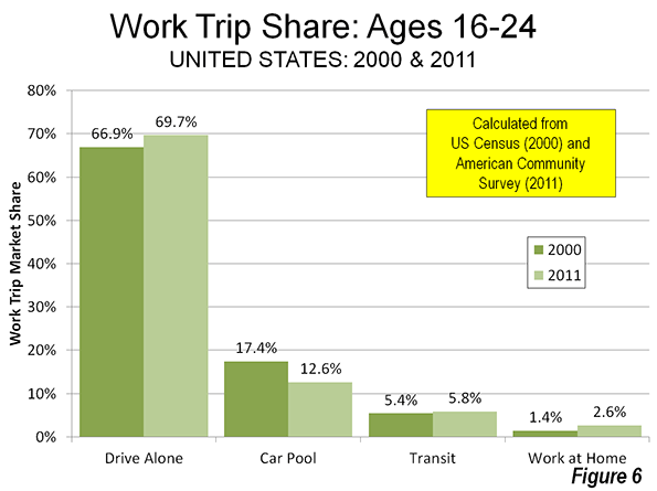
    In a widely cited study, Reid Ewing of the University of Utah, and UC Berkeley’s Robert Cervero reported only a minimal relationship between higher density and less driving per capita. In a meta-analysis of nine studies that examined the relationship between higher density and per household or per capita car travel, they found that for each 1 percent higher density, there is only 0.04 percent less vehicle travel per household (or per capita). This would mean that a 10 percent higher density should be associated with a reduction of 0.4 percent in per capita or household driving.

    More people in the same area driving a little less means overall driving is greater, as Peter Gordon reminds us. This is illustrated by the Ewing-Cervero finding — a 10 percent increase in population density is associated with  9.6 percent increase in overall driving, as is indicated in Figure 1 (the calculation is shown in the table). Ewing and Cervero placed this appropriate caution in their research: "we find population and job densities to be only weakly associated with travel behavior once these other variables are controlled."

    There is another limitation to the density-transit research. The comparison of travel behaviors between areas of differing density   provides no evidence that conversion of an area from lower to higher density would replicate the travel behavior of already existing (historic) areas of higher density.

    Transit is about Downtown, Not Density

    Ewing and Cervero also found that proximity to the central business district (downtown) is far more likely to reduce vehicle travel than higher densities. This mirrors the findings of others. The Ewing-Cervero conclusion is that, all things being equal, there is a 0.22 percent reduction in travel per capita for each one percent reduction in the distance to downtown.

    Table
    Density and Driving Example
      Base Density 1% Higher Density 10% Higher Density
    Households 100 101 110
       Change from Base Density 1.0% 10.0%
    Daily Driving per Household (Miles) 10 9.996 9.960
       Change from Base Density -0.04% -0.40%
    Total Daily Driving (Miles)        1,000       1,009.6           1,095.6
       Change from Base Density 0.96% 9.56%
    Based on Ewing & Cervero (2010)


    Transit commuting is strongly concentrated toward the largest downtown areas, which is the only place automobile-competitive mobility can be provided from large parts of the modern metropolitan area (whether in North America, Western Europe or Australasia).

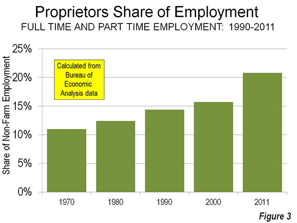
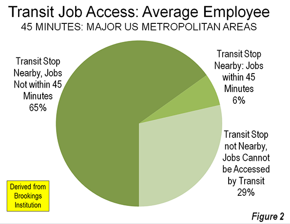
    This is, at least in part, why transit service provides such minimal employment access throughout major US metropolitan areas. Data from the Brookings Institution indicates that among the 51 metropolitan areas with more than 1,000,000 population, the average worker can reach only six percent of jobs in 45 minutes (see: Transit: The 4 Percent Solution). Nearly two-thirds of the jobs cannot be reached in 45 minutes, despite transit’s being nearby, while slightly less than one third of workers are not nearby transit at all (Figure 2). By comparison, the average driver reaches work in approximately 25 minutes.

    Of course, not everyone can (or would want to) live near downtown. Hong Kong comes closest to this urban containment ideal, with the highest population density of any major urban area in the high income world (67,600 per square mile or 26,100 per square kilometer).Yet despite these extraordinary densities,   one-way work trip travel times average 46 minutes, 20 minutes longer than in lower density, similar sized Dallas-Fort Worth.  

    High Density Commuting in the United States

    The centrality of downtown to transit ridership was a principal point of my “transit legacy city” research, which found that 55 percent of all transit commuting in the United States was to just six municipalities (not metropolitan areas). These include the municipalities of New York, Chicago, Philadelphia, San Francisco, Boston and Washington. Among the 55 percent of transit commuters in the nation who work in these six municipalities, 60 percent work in the downtown areas, which are the largest and most concentrated in the nation. This, combined with nearby high density neighborhoods, makes for transit Nirvana.

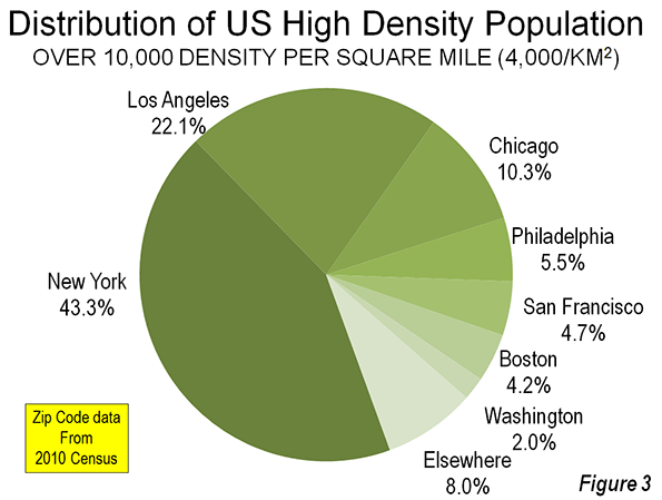
    The highest population densities are concentrated in just a few metropolitan areas (Note 2). Approximately 43 percent of the nation’s population living at or above 10,000 per square mile density (approximately 4000 per square kilometer) lives in the New York metropolitan area. Despite its low density reputation, Los Angeles has the second largest concentration of densities above 10,000 per square mile, at 22 percent. Chicago’s high density zip codes contain a much smaller 10 percent of the national high density population (Note 3), while nearly all of the balance is in Boston, San Francisco, Philadelphia, and Washington (Figure 3).

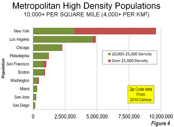
    The greatest concentration of the highest densities is in New York, which has 88 percent of the national population living at more than 25,000 per square mile (approximately 10,000 per square kilometer). Los Angeles ranked second at 3.5 percent and San Francisco ranks third at 3.2 percent (Figure 4). At this very high population density, nearly 60 percent of New York resident workers use transit to get to work. No one, however, rationally believes that densities approximating anything 25,000 per square mile or above will occur, no matter how radical urban plans become.

    An examination of transit work trip market shares in the density range of 10,000 per square mile to 25,000 per square mile illustrates the importance of proximity to downtown. There are nine metropolitan areas in the United States that have more than 200,000 residents living in zip codes with this density. These include the metropolitan areas with the six transit legacy cities, as well as Los Angeles, Miami and San Jose. These latter three experienced from two-thirds to 90 percent of their urban growth since World War II.

    San Jose’s large high density population is surprising, because it has a post-War suburban core city and, as a result, a comparatively weak downtown area. Moreover, San Jose has nearly 20 times as many people living at high densities as larger Portland, despite its more than three decades of densification policy (Note 4).

    Transit market shares are by far the highest in the high density zip codes of the metropolitan areas with the six transit legacy cities, at 30 percent. This ranges from 27 percent in Chicago to 33 percent in New York and Washington. At first glance, this would be evidence of a fairly consistent transit market share for high densities among the six metropolitan areas (Note 5).

    However, metropolitan areas containing the transit legacy cities are unique. Their high density areas are located near their large downtown areas (which are the largest and most concentrated employment centers in the nation), as is to be expected from urban forms that date from the 19th and early 20th centuries. The more recent urban forms of the metropolitan areas rounding out the top ten in high density residents, Los Angeles, Miami, San Jose and San Diego, are very different. Not only do they have smaller downtowns but their high density areas are not concentrated to the same degree around downtown. As a result, their high density transit work trip market shares are much lower (Figure 5).

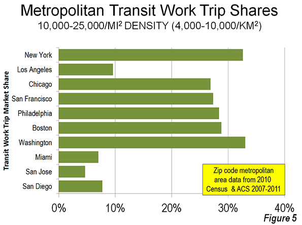
    This is best illustrated by Los Angeles, the metropolitan area with the largest number of people living at 10,000 to 25,000 residents per square mile in the nation. The transit work trip market share of these high density zip code residents is 9.6 percent, one-third that of similarly high densities in the metropolitan areas with transit legacy cities.

    In Miami, the transit work trip market share of high density residents is only 7.0 percent. In San Jose, the transit work trip market share for high density residents is only 4.6 percent, less than one-sixth that of the metropolitan areas with legacy cities. San Jose’s high density transit work trip market share is even below the national average for all densities (5.0 percent).  San Diego’s high density transit work trip market share is 7.7 percent.

    “A Negligible Impact”

    The transit-density disconnect may have been best summarized by Paul Shimik in 2007 research published in the Transportation Research Record: "The effect of density is so small that even a relatively large-scale shift to urban densities would have a negligible impact on total vehicle travel."

    Wendell Cox is a Visiting Professor, Conservatoire National des Arts et Metiers, Paris and the author of “War on the Dream: How Anti-Sprawl Policy Threatens the Quality of Life.

    —–

    Note 1: This article is limited to the potential for transferring automobile demand from cars to transit. Walking and cycling have only marginal potential for reducing vehicle travel, because these modes cannot provide access throughout today’s large metropolitan (labor) markets.

    Note 2: This analysis uses zip code level data from the 2010 Census and the American Community Survey for 2007-2011.

    Note 3: Los Angeles also has the second highest share of its population living at densities of 10,000 per square mile and above, at 38 percent. New York has 49 percent at this density, while in Chicago and San Francisco, 24 percent of residents live at these high densities.

    Note 4: Portland ranked 25th in high density (at or above 10,000 per square mile) out of the 51 metropolitan areas with more than 1,000,000 population in 2010. Portland’s high density share of its metropolitan population, at 0.7 percent, is well below that of the nation’s most market oriented development metropolitan area, Houston, at 2.0 percent and slightly below that of Dallas-Fort Worth.

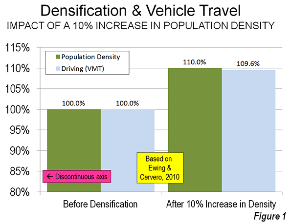
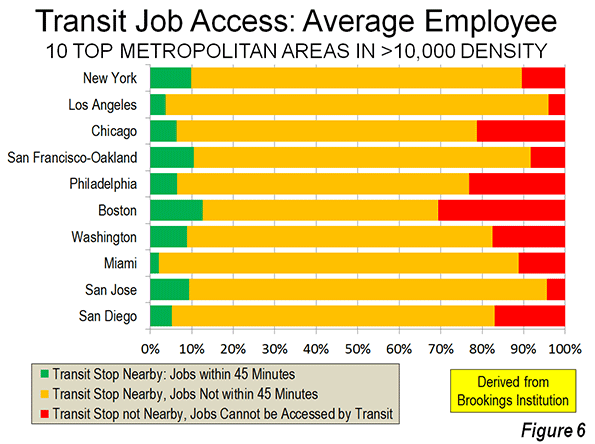
    Note 5: Despite their much higher transit work trip market shares in high density areas, the jobs in suburban areas in the metropolitan areas with legacy cities can be as inaccessible by transit as in the metropolitan areas with post-War core municipalities. See Figure 6.

    Photo: San Diego (by author)

  • US Sets New House Size Record in 2012

    There have been numerous press reports about the expansion of micro housing, and expectations that Americans will be reducing the size of their houses. As the nation trepidatiously seeks to emerge from the deepest economic decline since the 1930s, normalcy seems to be returning to US house sizes.

    According to the latest new single-family house size data from the US Census Bureau, the median house size rose to an all-time record of 2306 square feet in 2012. This is slightly above the 2277 square feet median that was reached at the height of the housing bubble in 2007 (Figure). The average new house size (2,505 square feet) remains slightly below the 2007 peak of 2,521 square feet.

    There was little coverage in the media, with the notable exception of Atlantic Cities, in which Emily Badger repeated the expectation of many:

    “It appeared after the housing crash that the American appetite for ever-larger homes was finally waning. And this would seem a logical lesson learned from a recession when hundreds of thousands of households found themselves stuck in cavernous houses they neither needed nor could afford.”

    But she concluded “Perhaps we have not changed our minds after all.” Well stated.

  • The Evolving Urban Form: The Rhine-Ruhr (Essen-Düsseldorf)

    Rhine-Ruhr, or Essen-Düsseldorf, is among the world’s least recognized larger urban areas (Figure 1).  Germany does not designate urban areas according to the international standard, and for that reason the Rhine-Ruhr does not appear on the United Nations list of largest urban areas. Yet, in reality this contiguous urban area is Germany’s largest urban area, a position as it has held since at least the end of World War II. The Rhine-Ruhr is the third largest urban area in Western Europe, trailing only Paris and London. The area was one of the strongest early urban industrial areas in the 18th century and continued as a major manufacturing and coal mining center through the first half of the 20th century.

    An Early Polycentric Urban Area

    The Rhine Ruhr is unusual in not having evolved around a single core municipality. The Rhine Ruhr has multiple core municipalities, which have grown together to form a conurbation, the second largest in the world following Osaka –Kobe – Kyoto. But the Rhine Ruhr is probably the most polycentric urban region in the world, with a minimum of eight older, large municipalities now linked by urbanization. These include Essen and Düsseldorf, which were until recently the two largest municipalities. In addition there are Dortmund, Duisburg, Bochum, Wuppertal, Gelsenkirchen and Oberhausen. Each of these eight municipalities reached a population of 250,000 or more by 1961.

    Like nearly all prewar municipalities in the high income world that had not expanded their boundaries, each of these has lost population since 1961. By 2011, the combined population of these eight municipalities was under 3.4 million, a reduction of 700,000 (Table) from their 1961 total (a 17% loss).

    Table
    Larger Rhine-Ruhr Municipalities: Population 1961-2011
      1961 2011 Change %
    Bochum      441,000      362,000     (79,000) -17.9%
    Dortmund      645,000      571,000     (74,000) -11.5%
    Duisburg      504,000      488,000     (16,000) -3.2%
    Dusseldorf      705,000      586,000   (119,000) -16.9%
    Essen      730,000      566,000   (164,000) -22.5%
    Gelsenkirchen      384,000      259,000   (125,000) -32.6%
    Oberhausen      258,000      210,000     (48,000) -18.6%
    Wuppertal      422,000      343,000     (79,000) -18.7%
    Total   4,089,000   3,385,000   (704,000) -17.2%


    Data for the balance of the urban area and the broader Rhine-Ruhr region (Note 1) is not readily available for 1961. As a result, this analysis considers the Rhine-Ruhr region to consist of the Dusseldorf, Arnsberg and Münster subregions of the state (lander) of North Rhine-Westphalia, which had a combined population of 11.22 million in 2011, up only modestly from 11.06 million in 1987. The urban area has a population of approximately 6.5 million residents, covering a land area of approximate 950 square miles (2,450 square kilometers). The urban density is approximately 6,800 per square mile (2,650 per square kilometers), less than that of Los Angeles (7,000 per square mile or 2,700 per square kilometer) or Toronto (7,600 per square mile or 2,900 per square kilometer).

    Since 1987, the Rhine-Ruhr has added 161,000 residents, having gained 617,000 residents between 1987 and 2001, and losing 456,000 from 2001 to 2011. The eight older cities lost 170,000 residents from 1987 to 2011, while the balance of the urban area lost 42,000. The exurbs, outside the urban area have added 373,000 residents, and account for more than all of the modest growth since 1987. All three sectors lost population after 2001 (Figure 2).

    Slow Growth, Even for Germany

    The Rhine-Ruhr is located in the lander of North Rhine-Westphalia, which has the largest population in Germany. Its growth, however, has been glacial. Since 1961, the average annual growth rate of the lander was 0.2%. This is one third the growth rate of the other lander that constituted the former Federal Republic of Germany (West Germany).

    North Rhine-Westphalia’s performance is stellar compared to the lander of the former Democratic Republic of Germany (East Germany), which have fallen back to their 1961 population, having lost 10% of their residents since 1990. Germany itself lost more than 2 million people in the last decade, reflecting its well-below replacement fertility rate. Based upon this rate, Germany could lose more than the 5 million more residents projected by United Nations projectionsto 2050 (to 75 million).

    But even within the slow growth environment of North Rhine Westphalia, the  Rhine Ruhr region is falling behind as nearly all the growth has shifted elsewhere to the regions of the lander that surround other urban areas, Cologne (Köln), which includes the former West German capital of Bonn, and Aachen (which stretches into the Netherlands). Local authorities in the Ruhr Valley are forecasting a population loss of approximately 8 percent by 2030.

    The Setting

    The Rhine-Ruhr conurbation is organized around confluences of two rivers with the Rhine. The northern part of the urban area stretches from the west bank of the Rhine eastward along the Ruhr River Valley with the large municipality of Duisburg anchoring the West and Dortmund the East. The southern part of the urban area stretches along the Wupper River Valley starting at Düsseldorf and continuing eastward to south of Dortmund. The elevation at the two river junctions is less than 100 feet (40 meters). A transverse, low mountain range (Rhenish Massif) separates the northern and southern parts of the urban area (maximum elevation 800 feet or 300 meters), though much of the hilly area is urban.

    Transport

    Without a dominant, large center, the Rhine-Ruhr has a lower transit work trip market share – 18 percent – than would be expected for a European urban area of its size. This is well below the 30 percent share of Berlin and the approximately 35 percent shares of Madrid, Lisbon, and Stockholm, which are all smaller than the Rhine-Ruhr. Wuppertal is home to one of the icons of mass transit, the Wuppertal Monorail, which opened in 1901. The Monorail is suspended for much of its route above the Wupper River, with supports straddling the river (such a configuration would probably not be permitted to be constructed today in any high-income world metropolitan area because of environmental regulations).

    The Rhine-Ruhr’s polycentricity requires substantial reliance on its road system. The region is well served by an extensive freeway (autobahn) system consisting of at least four east-west routes and five north-south routes. Traffic congestion is worse than in most US urban areas, but the Rhine-Ruhr’s traffic flows better than in any metropolitan area of similar size in Europe, according to 2012 data from the INRIX Traffic Scorecard. The average peak hour delay is 14.8 percent compared to “free flow.” This is less than one-half the average delay in smaller Milan (30.2 percent) and well below Paris (27.8 percent) and London (26.1 percent). In 2005, the Rhine-Ruhr had the fifth highest rated freeway access among 30 surveyed international urban areas.

    Shrinking City

    Shrinking cities (where cities are defined as metropolitan areas or urban areas) have been unusual in the high income world (Pittsburgh and Liverpool are exceptions). Even as core municipalities have lost population, such as in Atlanta and Copenhagen, metropolitan areas have continued to grow. This is likely to change because of the severe national population declines forecast in a number of countries. The Rhine-Ruhr, and other similarly situated cities, will face serious challenges in retaining dynamic economies and delivering public services in the years to come for an aging population supported by a smaller work force.

    Wendell Cox is a Visiting Professor, Conservatoire National des Arts et Metiers, Paris and the author of “War on the Dream: How Anti-Sprawl Policy Threatens the Quality of Life.

    ———–

    Note 1: The entire Rhine-Ruhr and Cologne areas are considered by Germany to be the Rhine-Ruhr metropolitan area (ballungsräume). This article is limited to an area roughly conforming to the northern part of the ballungsräume. Eurostat defines a much smaller Düsseldorf-Ruhrgebiet metropolitan area that includes the Rhine-Ruhr urban area and most of the exurban area in this analysis. There is no international standard for the designation of metropolitan areas (labor markets).

    Note 2: INRIX classifies the Rhine-Ruhr as two areas (north and south). This is the population weighted congestion delay.

    Photo: Wuppertal Monorail

  • An Economics Lesson from The New York Times

    The New York Times restates basic economics in a June 9 editorial that should be required reading for planners and public officials who fail to comprehend how restrictions on housing raise prices. The Times expressed concern about the extent to which investor involvement in some markets has raised the price of houses for new homebuyers and others who actually plan to live in the houses that they purchase. The price increasing impact of excess demand on housing markets from institutional investors is no different what occurs when urban planning policies restrict housing supply, as occurs with urban containment policy.

    Referring to the recent house price increases, The Times said “Those gains, in turn, have propelled rising home prices nationwide, in part by reducing supply and in part by fostering a shift in perceptions about the housing market that has drawn some potential home buyers off the sidelines.” In this, The Times simply expresses the economic reality that when demand exceeds supply, house prices (or any other prices), other things being equal, will tend to rise. The cause of the imbalance is of no account.

    But The Times did not limit its analysis to economics. Venturing into the social dimension, The Times went so far as to endorse home ownership: “Given the traditional role of homeownership in building wealth, fostering communities and driving the economy forward, a lower rate of homeownership is a troubling development.”

    The Times editorial board has taken a position challenging the agendas of some of the most prominent retro-urbanist theorists, who favor more renting and less home ownership, clinging to the fantasy that, somehow housing markets constrained by excessive planning regulations are exempt from the laws of supply and demand.

  • Canada’s Central Bank Issues Warning on Toronto Condominium Market

    For a few years, concern has been expressed about house price increases in Canada, which have been disproportionate compared to household incomes.

    In this regard, the latest, semi-annual Bank of Canada Financial System Review points to the overbuilt multi-unit market, especially the Toronto condominium market, as having the potential to inflict serious harm on the economy (see A Toronto Condo Bubble?), including “reduced household net worth.” In its report, Canada’s central bank said:

    “…the total number of housing units under construction remains significantly above its historical average relative to the population. This development is almost entirely attributable to multiple-unit dwellings (which include condominium units). In the Toronto condominium market, the number of unsold high-rise units in the pre-construction and under-construction stages has remained near the high levels observed since early 2012. If the investor component of demand has boosted construction in the condominium market beyond demographic requirements, this market may be more susceptible to shifts in buyer sentiment. Furthermore, if the upcoming supply of units is not absorbed by demand as they are completed over the next 12 to 30 months, the supply-demand discrepancy would become more apparent, increasing the risk of an abrupt correction in prices and residential construction activity.

    Any correction in condominium prices could spread to other segments of the housing market as buyers and sellers adjust their expectations. Such a correction would reduce household net worth, confidence and consumption spending, with negative spillovers to income and employment. These adverse effects would weaken the credit quality of banks’ loan portfolios and could lead to tighter lending conditions for households and businesses. This chain of events could then feed back into the housing market, causing the drop in house prices to overshoot.

    (Emphasis by author)

    Canadian analysts have long been concerned about the potential for its rising house prices to collapse, as occurred in the overheated US markets. Just as the housing bust in California, Florida, Arizona and Nevada threw the US economy and that of the world into the worst economic decline since the Great Depression, a housing price bust could inflict serious damage to the Canadian economy, which has performed strongly in recent years.

    In the United States, the housing bust led to a nearly 20 percent reduction in household net worth, while recent reports show that the loss has been recovered. However, this recovery has been anything but equal. Many households who suffered losses, such as in investments intended to finance retirement, have not seen their wealth restored.

    There is plenty about housing market distortion for Canada to be concerned about.

  • Toward a Self Employed Nation?

    The United States labor market has been undergoing a substantial shift toward small-scale entrepreneurship. The number of proprietors – owners of businesses who are not wage and salary employees, has skyrocketed, especially in the last decade. Proprietors are self employed business owners who use Internal Revenue Service Schedule C to file their federal income tax. Wage and salary workers are all employees of any establishment (private or government), from executives to non-supervisory workers.

    From 2000 to 2011, the number of non-farm proprietors grew by 10.7 million. Total wage and salary employment grew by only 105,000 between 2000 and 2011. Government employment, including federal, state and local, grew 1.36 million, while private employment declined by 1.26 million (Figure 1).

    As a result, 99 percent of the total increase in employment from 2000 to 2011 was in the self-employed, according to Bureau of Economic Analysis of the United States Department of Commerce data. By comparison, during the 1990s, self employment accounted for only 22 percent of the increase in jobs nationally (Figure 2). The economic impact of the increase in self employment may be less, however, than its gross numbers, because many of the self employed are also engaged in wage and salary employment (Note).

    Self Employment Gains in the Great Recession

    Perhaps most striking is the fact that the number of entrepreneurs continued to grow in the Great Recession and what might be called the continuing Great Malaise. From 2007 to 2011, there was an increase of 1.8 million proprietors. This annual growth of nearly 450,000 was more modest than between 2000 and 2007, when the average number of proprietors grew 1.28 million, nearly three times as fast. The continuing growth in proprietors starkly contrasts with the loss of 5.9 million in private sector jobs. Government employment grew 44,000.

    A Longer Term Trend

    The data from 2000 to 2011 indicates an acceleration of an already developing trend of greater self employment, which can be traced back to at least 1970 (the earliest data readily available). In 1970, proprietors were 11.0 percent of employment, a figure that rose to 15.6 percent by 2000. The greatest increase occurred after 2000, when the number of proprietors increased 42 percent. In 2011, proprietors represented 21 percent of employment, nearly double their proportion in 1970 (Figure 3).

    This increase in proprietors (and their generally smaller commercial establishments) tracks with the continuing decline in average establishment size (Figure 4). United States Bureau of Labor Statistics data shows that between 2002 and 2012, there was a loss of 2.3 million private jobs in establishments with 100 or more employees. Establishments with 500 or more employees experienced a reduction of 1.8 million jobs, 80 percent of the large establishment (100 and over) losses. These losses were nearly made up by gains in establishments with under 100 employees (2.1 million).

    State Self Employment Trends

    Self employment added the largest number of jobs in 40 states between 2000 and 2011 (Table). Its percentage increase exceeded both those of private and government employment in all but two states (North Dakota and Alaska)

    Texas added the largest number of proprietors between 2000 and 2011. The Lone Star state added 1.26 million proprietors. Florida ranked second, added 970,000 proprietors, followed by California with 940,000. New York with its long laggard economic growth , added 820,000 proprietors. Georgia ranked 5th, adding 540,000. The next five included fast growing North Carolina (8th), as well as slower growing New Jersey, Illinois, Pennsylvania and Michigan (yes, Michigan).

    The story, however, was much different among these states in wage and salary employment. Texas, with the nation’s most vibrant and business friendly big state economy (according to chiefexecutive.net), added 1.22 million wage and salary jobs, 960,000 of which were in the private sector. Florida did somewhat worse, adding only 201,000 jobs, 113,000 in the private sector. California lost 480,000 private sector jobs, while adding 62,000 government jobs. Public and government employment changed little in New York. Georgia lost 131,000 private jobs, while adding 87,000 to government payrolls, while New Jersey and Illinois suffered private sector losses of 155,000 and 355,000 respectively (Figure 5 and Table).

    EMPLOYMENT CHANGE BY TYPE OF JOB: 2000-2011
    Wage & Salary Employment Total Employment
      Private Government Total Proprietors
    Alabama            (69,050)          22,297        (46,753)          154,522           107,769
    Alaska             39,839          12,355         52,194             9,621             61,815
    Arizona            126,805          51,509       178,314          245,934           424,248
    Arkansas              (8,806)          27,902         19,096           47,141             66,237
    California           (479,691)          62,143      (417,548)          941,071           523,523
    Colorado              (8,740)          70,077         61,337          209,084           270,421
    Connecticut            (64,857)            3,022        (61,835)          168,636           106,801
    Delaware            (11,550)            6,597         (4,953)           35,349             30,396
    District of Columbia             46,402          27,180         73,582           29,288           102,870
    Florida            113,353          88,063       201,416          968,006        1,169,422
    Georgia           (131,337)          87,525        (43,812)          537,451           493,639
    Hawaii             33,157          17,126         50,283           35,638             85,921
    Idaho             37,459            8,327         45,786           54,325           100,111
    Illinois           (354,730)           (5,481)      (360,211)          374,270             14,059
    Indiana           (180,865)          18,415      (162,450)          105,068            (57,382)
    Iowa             10,472          11,440         21,912           49,320             71,232
    Kansas            (17,794)          21,022          3,228           74,747             77,975
    Kentucky            (48,771)          39,826         (8,945)           86,259             77,314
    Louisiana               8,380         (16,543)         (8,163)          219,700           211,537
    Maine            (11,858)            1,060        (10,798)           23,994             13,196
    Maryland             28,580          54,102         82,682          249,229           331,911
    Massachusetts            (96,684)           (4,699)      (101,383)          211,607           110,224
    Michigan           (666,239)         (66,184)      (732,423)          294,215          (438,208)
    Minnesota              (3,680)            6,886          3,206          155,151           158,357
    Mississippi            (64,479)            5,696        (58,783)           87,067             28,284
    Missouri           (107,603)          12,903        (94,700)          138,189             43,489
    Montana             38,149            7,163         45,312           31,068             76,380
    Nebraska             15,922          12,470         28,392           42,849             71,241
    Nevada             75,814          35,526       111,340          136,382           247,722
    New Hampshire              (7,892)            9,275          1,383           41,525             42,908
    New Jersey           (155,108)          21,622      (133,486)          405,353           271,867
    New Mexico             48,017          11,506         59,523           37,120             96,643
    New York               2,427           (5,997)         (3,570)          818,861           815,291
    North Carolina            (58,042)        121,486         63,444          329,109           392,553
    North Dakota             65,306            7,595         72,901           15,776             88,677
    Ohio           (514,436)           (5,380)      (519,816)          277,931          (241,885)
    Oklahoma             28,310          41,462         69,772          106,262           176,034
    Oregon             19,047          16,878         35,925           95,406           131,331
    Pennsylvania            (11,087)          17,678          6,591          310,306           316,897
    Rhode Island            (15,349)           (4,281)        (19,630)           29,356              9,726
    South Carolina            (42,912)            9,998        (32,914)          242,447           209,533
    South Dakota             28,301            7,155         35,456           20,290             55,746
    Tennessee            (84,441)          33,905        (50,536)          196,021           145,485
    Texas            956,988        264,871    1,221,859       1,255,773        2,477,632
    Utah            109,728          33,864       143,592          137,781           281,373
    Vermont              (4,419)            4,179            (240)           21,467             21,227
    Virginia             90,766          64,639       155,405          282,009           437,414
    Washington             77,224          62,267       139,491          170,512           310,003
    West Virginia               8,796            9,736         18,532           20,765             39,297
    Wisconsin            (81,794)          13,783        (68,011)          148,572             80,561
    Wyoming             33,972          10,034         44,006           21,077             65,083
    United States        (1,259,000)     1,364,000       105,000     10,698,900      10,803,900

    The Future?

    Robert Fairlie, one of the nation’s leading experts on self-employment and a professor at the University of California, Santa Cruz, associates much of the increase in proprietors during the Great Recession to higher unemployment rates, measured at the local level. This is consistent with the rise in self employment during the Great Recession and the huge wage and salary job losses. At the same time, the larger increases in the decade before the Great Recession may indicate a strong underlying trend toward self employment. Certainly, this is supported by the rise of the Internet, which provides cheaper access to information and more comprehensive marketing opportunities.

    The future could see stronger self employment gains. As the baby boom generation reaches retirement age, it is likely that many former employees will turn to self employment to increase their incomes.

    Finally, the increasing global competitiveness could continue to reduce establishment sizes and encourage greater self employment. Stronger business regulation, including the mandates of the new medical care system ("Obamacare") could result in stunted employment growth, or even losses, forcing more people into self-employment even if they continue to work with current employers as contractors.

    America may not become a "nation of shopkeepers," like 19th century Britain, but is   increasingly becoming a self-employed nation. It will be challenging for governments, both at the national and local level to develop regulatory and tax structures that encourages this entrepreneurial expression, and perhaps more problematic, figure out to aid their conversion into larger businesses.

    Wendell Cox is a Visiting Professor, Conservatoire National des Arts et Metiers, Paris and the author of “War on the Dream: How Anti-Sprawl Policy Threatens the Quality of Life.

    —-

    Note: This article uses Bureau of Economic Analysis employment counts — the number of jobs, rather than employees (an employee may have more than one job). The database in this analysis includes full and part time employment. Last year’s Forbes article used a different database, limited to people who make their livings principally from self employment.

    Self employment photo by BigStockPhoto.com.

  • Driving Trends in Context

    There are grains of reality, misreporting and exaggeration in the press treatment of a report on driving trends by USPIRG. The report generated the usual press reports suggesting that the millennial generation (ages 16 to 35) is driving less, moving to urban cores, and that with a decline in driving per capita, people are switching to transit. These included the usual, but not representative anecdotes about people whose lifestyles and mobility needs are sufficiently served by the severe geographical and travel time limitations of transit.

    Further, in an important contribution, the USPIRG report provides driving trend forecasts that are lower than other projections. If accurate, these would result in materially greater greenhouse gas emissions reductions to 2040 than projected by the Department of Energy, further undermining the justification for anti-mobility policies as well as urban containment.

    Millennials and More Urban and Walkable Living

    It is again reported that millennials "like to live in the city center." Last year, a report by USPIRG cited a poll indicating that 77 percent of millennials plan to live in urban cores. Their actual choices have been radically different.

    In fact, 2010 census data indicates that people between 20 and 29 years old were less inclined to live in more urban and walkable neighborhoods than their predecessors. In 2000, 19 percent of people aged 20 to 29 lived in the core municipalities of major metropolitan areas, where transit service and walkable neighborhoods are concentrated. Only 13 percent of the increase in 20 to 29-year-old population between 2000 and 2010 was in the core municipalities. By contrast, the share of the age 20 to 29 living  in the suburbs of major metropolitan areas was 45 percent, higher than the 36 percent living there in 2000 (Figure 1).

    The Decline in Driving

    Driving per capita in urban areas peaked in 2005. Between 2005 and 2011, driving declined seven percent. In the context of rising gasoline prices, and economic trends, the real news is not how much driving has fallen, but rather how little. A seven percent reduction is slight compared to the one and one-half times increase in gas prices over the past decade (Figure 2). Per capita travel by car and light truck has fallen back only to 2002 levels, which remained above the driving rates of previous years.

    Drivers: Not Switching to Transit

    The USPIRG report gives the impression that instead of driving, Americans are switching to other modes of transport, principally transit. In discussing the report, Nick Turner, of the Rockefeller Foundation said: "Americans are making very different transportation choices than they did in years past."

    Actually not. The data shows that as people drove less, they did not switch to transit. The driving reduction was approximately 900 miles per capita from 2005 to 2011. At the same time, transit ridership per capita was up approximately 15 miles – a small change compared to the reduction in driving (Figure 3). People just traveled a less (perhaps fewer trips to the store or to the beach, not to mention the fewer work trips in a depressed economy).

    Work trip travel trends are little changed over the past decade. Driving alone and transit were up marginally between 2000 and 2011. Working at home increased the most, while car pooling declined the most (Figure 4).

    This raises the issue of context. While driving was declining about seven percent per capita from 2005 to 2011, transit use was increasing about seven percent. The percentages were similar, but the amount of travel was radically different, because of transit’s much smaller base. Transit usage would need to increase nearly 400 percent to equal the mileage of a seven percent loss in travel by car. For all of the impressive transit ridership increase claims, transit’s share of urban travel has changed little (Figure 5).

    Transit’s failure to capture much of the decline in driving simply reflects the limitation of its effectiveness in taking people where they need to go. Transit is very effective in providing mobility to the nation’s largest downtown areas, where it provides half to three quarters of the trips. Approximately 55 percent of all US transit commuting is to six transit legacy cities (municipalities), including New York, Chicago, Philadelphia, Boston, San Francisco, and Washington. Most of this commuting is to the compact and dense downtown areas.

    Outside the transit legacy cities, transit’s impact is slight, because of the "last mile" problem.  Transit service is not close enough (or fast enough) to be practical for most trips in metropolitan areas. For example, Brookings Institution data indicates that the average worker can reach fewer than 10 percent of of jobs in major metropolitan areas within 45 minutes. By contrast, the average solo driver reaches work in approximately 25 minutes. There is no solving this problem, because the infrastructure that would be required is far from affordable, as Professor Jean-Claude Ziv and I showed in a WCTRS paper (See: Megacities and Affluence).

    Millennial Driving in Context

    Survey data does indicate a decline in driving among millennials, but those with jobs are not flocking to transit. Single occupant commuting in this age group increased between 2000 and 2011, from 66.9 percent to 69.7 percent. Transit use and working at home also increased (5.4 percent to 5.8 percent and 1.4 percent to 2.6 percent respectively. There was, however, a substantial decline in car pool use among millennials, from 17.4 percent to 12.6 percent (Figure 6).

    Younger workers have suffered disproportionately from the economic decline. There has been a substantial reduction in the percentage of people aged 16 to 24 who have jobs (Figure 7). These lost work trips have contributed more than any perceived preference for urban living to the decline in driving. Transportation expert Alan Pisarski has attributed much of the decline in demand in this age group to such economic factors.

    At the same time, and as USPIRG indicates, the increase in social media use may well have contributed to the declining demand for discretionary travel.

    Driving Less in the Future and the GHG Emissions Implications

    The decline in per capita driving is not surprising. Back in 1999, Pisarski predicted that per capita driving would soon peak ("Cars, Women and Minorities: The Democratization of Mobility in America"), because automobile availability had now spread to most all segments of society.

    USPIRG forecasts driving volumes below US Department of Energy predictions. According to USPIRG:  "Coupled with improvements in fuel efficiency, reduced driving means Americans will use about half as much gasoline and other fuels in 2040 than they use today." This means an even greater reduction in GHG emissions than currently forecast. Department of Energy forecasts a 21 percent decline in total (not per mile) GHG emissions from light vehicles between 2010 and 2040, despite a 40 percent increase in driving. The more modest driving levels in USPIRG scenarios would result in GHG emissions reductions of between 31 percent and 55 percent between 2010 and 2040 (Figure 8). These projections provide further evidence that of the "greening" of the automobile and the needlessness of urban containment policies.

    Reality

    Regardless, however, of the future trend, it is important to minimize the time that people spend traveling in metropolitan areas, because of the strong association between effective mobility, job access, and economic growth. Modern metropolitan areas require the quickest possible access between all origins and destinations to facilitate greater household affluence (measured in discretionary income) and lower levels of poverty. The objective should be the greatest reduction in travel delay per dollar spent on transportation.

    Dug Begley accurately characterized the situation in the Houston Chronicle:

    "We spend a lot of transportation money in the Houston region on roads, and for good reason: That’s how most people travel. Houston is a growing place, and there aren’t two or three job centers, there are about eight. Getting people between them … is going to take roads."

    Outside the municipal boundaries of the six legacy cities and especially their downtown enclaves, Houston (despite its reputation) is little different than the rest of metropolitan America. From the suburbs of New York, to the entire Portland and Phoenix metropolitan areas, the automobile carries the overwhelming share of travel (see Table 1, here). It cannot be any other way, since no planning agency in the New World or Western Europe has a plan, much less the resources, to construct a transit system that would duplicate the mobility of the automobile throughout its metropolitan area.

    Wendell Cox is a Visiting Professor, Conservatoire National des Arts et Metiers, Paris and the author of “War on the Dream: How Anti-Sprawl Policy Threatens the Quality of Life.

    —–

    Methodology: This article is based on data from the Federal Highway Administration, the Federal Transit Administration, Census Bureau, Department of Energy and USPIRG.

    Photo: Roadways, Fort Lauderdale (Miami metropolitan area)