Author: Wendell Cox

  • Australia Central Banker: Higher House Prices a “Social Problem”

    Glenn Stevens, the Governor of the Reserve Bank of Australia expressed concern about the growing gap in housing affordability in the nation to a parliamentary committee on Friday. Stevens raised questions about the cost and supply of housing, asking:

    "How is it that we can’t add to the dwelling stock for the marginal new entrant more cheaply than we seem to be able to do," he asked.

    According to an article in the Perth Western Australian ("High price of homes ‘stealing future’") Stevens went on to say that key State and local government issues around supply, zoning, transportation and infrastructure seemed to be making a simple block of land more expensive than was necessary.

    Virtually all of Australia large urban areas have implemented urban containment policies (called "urban consolidation" in Australia and "smart growth" in the United States). The result has been to increase house prices from 2 to 3 times the historic norm relative to incomes. These price increases are consistent with the overwhelming economic evidence of a strong association between urban containment policies, especially those that ration land for development through devices such as urban growth boundaries.

    The Chairman of the Reserve Bank of New Zealand has identified a 10-times "across the urban growth boundary value" difference per acre in Auckland, which is similar to findings in Portland, Oregon.

    Stevens concluded his housing comments noting that: "There’s a very big inequality between generations building up and I think that’s a social problem as much as any economic point."

  • New Zealand Leader Focuses on Association between High House Prices and Growth Management

    ACT Party leader Donald Brash, who served from 1988 to 2002 as the Governor of the Reserve Bank of New Zealand (similar in function to the Federal Reserve Board) has noted the poor housing affordability in New Zealand and its connection to growth management policies (called by various names, such as "smart growth," "growth management," "compact cities," "densification" "prescriptive land use regulation" and "urban consolidation").

    In an August 25 speech Brash said:

    "It is impossible to avoid the conclusion that the interaction of the RMA, the Local Government Act and local government staff all over the country has produced a major obstacle to improved living standards.

    One of the ways this has happened is through the way in which this interaction has pushed the price of housing well beyond the reach of far too many New Zealanders – or more accurately, has pushed the price of residential land well beyond the reach of far too many New Zealanders.

    We know, from the annual surveys undertaken by the Demographia organisation, that housing in our major cities is now among the most expensive in the world, relative to household incomes. And why? In large part because too many local governments have quite deliberately limited the supply of residential land.

    Arthur Grimes, now chairman of the Reserve Bank, found that the effect of the Metropolitan Urban Limit imposed by the Auckland Regional Council had increased the price of land just inside that Limit by some 10 times compared with the price of land just outside the Limit.

    This is absolutely nuts, in a situation where New Zealand is one of the most under-populated countries in the world, and where Auckland is one of the most densely populated cities in the world – in terms of people per square kilometre, Auckland is more densely populated than Vancouver, Melbourne, Portland, Adelaide, Perth or Brisbane.

    I’m delighted that one of the first projects of the newly-established Productivity Commission is to look into the affordability of housing."

    The finding of a 10-times "across the urban growth boundary value" difference per acre in Auckland, is similar to findings in Portland, Oregon.

    Dr. Brash had previously written (the "Median Multiple is a measure of housing affordability, with higher number indicating less affordable housing. It is the median house price divided by the median household income):

    "… the one factor which clearly separates all of the urban areas with high Median Multiples from all those with low Median Multiples is the severity of the artificial restraints on the availability of land for residential building"

  • Suburbanized Core Cities

    The suburbs of major metropolitan areas captured the overwhelming majority of population growth between 2000 and 2010, actually increasing their share of growth, as has been previously reported. However, it is often not understood that much of the recent central city (Note 1) growth has actually been suburban in nature, rather than core densification. In fact, historical core cities (Note 2) vary substantially. In some cases, core cities are largely pre-war and transit oriented, such as New York, Chicago and San Francisco. In other cases, much of historical core city is automobile oriented suburban in character. This article provides a classification of historical core cities based upon the extent of their pre-automobile cores as well as population and land area data.

    Central Cities before World War II: Auto-oriented suburbanization began before the Great Depression.  In 1940, transit’s urban market share in the United States appears to have been higher than that of Western Europe today (Note 3). Each of the nation’s largest metropolitan areas (then called "metropolitan districts") boasted a strong, dense core, and could be generally delineated by the city limits of the largest municipality.

    In the years after the Second World War, many cities annexed considerable territory. At the same time, a number of new major metropolitan areas emerged which effectively lacked a dense core. For the purposes of analysis, the historical core cities of the 51 major metropolitan areas (those with more than 1,000,000 population) have been divided into three categories, based upon the extent of the suburban development within their borders. The categories are defined in Table 1 and data is provided in Tables 2 and 3 in the attached PDF document.

    Table 1
    Classification of Historical Core Municipalities

    Nature of Historical Core Municipality:
    Classification based upon 2010 City Limits

    Large Urban Core in 1940?

    2010
    City Limits

      Pre-War & Non-Suburban

    Yes

     Is pre-war core; nearly all included land area was developed by 1940. Little development that is post-war suburban in character. Little or no change in boundaries since 1940.

      Pre-War  & Suburban

    Yes

    Includes pre-war core, however contains substantial development that is post-war suburban in character (2010 boundaries contain substantial areas that were greenfield in 1940)

      Post War & Suburban

    No

    Has smaller pre-war core: less than 100,000 population in 1940 and nearly all development is post-war suburban in character.

    The historical core municipality is the municipality with the largest 1940 population in the present metropolitan area (metropolitan statistical area).
    There can be more than one historical core municipality in a metropolitan area, with the exception below.
    There can be a second historical core municipality if (1) it is adjacent to a historical core municipality classified as "Pre-War  & Non-Suburban," (2) had a 1940 population at least 25 percent of the first historical core municipality and (3) a population density of at least 5,000 per square mile.
    Multiple municipality names listed in some other metropolitan areas for reference purposes.

    Pre-War & Non Suburban: The first category is the "Pre-War & Non Suburban" historical core cities. Each of these 19 cities is itself a pre-automobile core. City boundaries have changed little since before World War II and nearly all land was developed at that time (Note 3).

    Overall, these cities had a population density of 11,900 per square mile in 2010 (Figure 1). However, 16 of the cities have lost population since 1940, with only New York, San Francisco and Oakland having gained population, albeit very modestly. (Oakland lost population over the past decade.) Between 2000 and 2010 the "Pre-War & Non Suburban" historical core cities lost 424,000 people, or 2.2 percent of their population (Figures 2 and 3). Seven gained population, though in five of these cases (Boston, Hartford, Philadelphia, Providence and Washington) the 2010 population remained well below mid-century levels.

    Pre-War & Suburban: The second category is the "Pre-War & Suburban" historical core cities. These 27 cities had pre-automobile cores, usually quite small, in 1940, but also include (in their 2010 borders) substantial land that was undeveloped in 1940. Substantial automobile-oriented suburban development has occurred in these areas. The strong automobile oriented suburban influence is indicated by the average population density of 2900 people per square mile of land area, approximately one-fourth the density in the "Pre-War & Non Suburban" category.

    On average, the 2010 land area of the "Pre-War & Suburban" historical core cities is 3.2 times the land area of the corresponding urban areas in 1950 (areas of continuous development or the "urban footprint"). These urban areas included both the historical core city and the suburbs (Note 4).   The city of Jacksonville covers the most land area relative to its 1950 urban area, at 14.7 times. The city of Portland, the recipient of frequent praise by advocates of densification, covered more area in 2010 than its entire urban area in 1950 and its population density today is less than that of the entire urban area in 1950.

    The "Pre-War & Suburban" historical core cities added 1,520,000 people between 2000 and 2010. This translates into an average growth of 7.8 percent relative to the 2000 population. Three cities grew more than 100,000. Louisville added 341,000 people principally through a city – county merger, after its previous annexations had failed to stop its population decline. Between 1950 and 2000, Louisville has lost nearly one-third of its population while adding more than 50 percent to its land area.

    Charlotte added 191,000 people, principally due to a continuing annexation program. San Antonio and Houston took advantage of considerable undeveloped land within their city limits to add 183,000 and 146,000 people respectively.

    Post-War & Suburban:  The third category is the "Post-War & Suburban" historical core cities. None of these seven cities had more than 100,000 population in 1940 or a large pre-automobile core; these are essentially suburbanized cities.  In each case, the cities have undertaken huge annexations. On average, the 2010 city limits include nearly 6 times as much land as the corresponding urban areas in 1950. The city of San Jose, known for its densification policies, covers nearly 3 times as much land as its entire urban area in 1950, which included the city and all of the suburbs (Figure 4).

    The "Post-War & Suburban" historical core cities added 619,000 people between 2000 and 2010, for an increase rate of 15.5 percent, the largest percentage growth of the three categories.

    Perhaps surprisingly the population density of the "Post-War & Suburban" historical core cities was one-quarter above that of the "Pre-War & Suburban" category, at 3700 per square mile. This may be at least partially driven cities like San Jose, Las Vegas and Riverside-San Bernardino, which have generally avoided planning that required larger lots and below market densities.

    The cities of Philadelphia and Phoenix reflect these differing patterns.   In 2010 Philadelphia had a population density of more than 11,300 people per square mile and covered an area of 135 square miles. The city of Phoenix had a population density of under 3000 people per square mile and covered more than 500 square miles. Not even one square mile of the 2010 city of Phoenix equals the average density of Philadelphia. In 1940, Philadelphia had a population of 1.9 million, 30 times that of the 65,000 in Phoenix.

    As would be expected in a dense historic core city, Philadelphia has a substantial transit work trip market share, at 25 percent. This is five times that of the surrounding suburbs (5 percent). In contrast, the city of Phoenix has s a transit work trip market share of only three percent, below that of the Philadelphia suburbs. 

    Suburban Development Makes Cities Grow: As the data above indicates, virtually all net core city population growth over the past decade has been suburban in nature. Core cities characterized by substantial automobile-oriented suburbanization added more than 2.1 million residents, while the cities with little   automobile-oriented suburbanization lost more than 400,000. It turns out that even most “core” cites are more suburban than many imagine.

    ——————–

    Note 1: "City" has multiple meanings and analysts have not always provided  sufficient clarity when using the term. For example, "city" can mean a metropolitan area, and urban area, a municipality (incorporated jurisdiction) or as in China, a region either at the provincial or sub-provincial level. As used in this article, the term "city" means a municipality unless otherwise indicated.

    Note 2: The historical core city is the city in the present metropolitan area that had the largest population in 1940. Usually, this is the first named city in the official Census Bureau title. However, in two cases (Virginia Beach-Norfolk and Riverside-San Bernardino), the second named city is the historical core city because it was the largest in 1940.

    Note 3: There are no comparable data on overall transit market shares between Europe and the United States. However, Eurostat data for nearly 150 European metropolitan areas indicates that transit’s work trip market share averages approximately 17 percent. The same population range (over 100,000) of US metropolitan areas has a transit work trip market share of six percent. In 1940, the overall US transit market share was approximately 14 percent. Because transit work trip market shares are generally substantially higher than overall shares, it is suggested that the 1940 US transit market share was greater than the current share in Europe.

    Note 4: The city of Chicago made a substantial annexation largely to incorporate the land for O’Hare International Airport. This annexation did not materially increase post-war suburban development in Chicago and the city is thus classified as "Pre-War & Non-Suburban."

    Note 5: 1950 used because urban areas were not designated before that time.

    Wendell Cox is a Visiting Professor, Conservatoire National des Arts et Metiers, Paris and the author of “War on the Dream: How Anti-Sprawl Policy Threatens the Quality of Life

    Photo: City of San Antonio annexation map from the San Antonio Planning and Development Department. The red rectangle is the land area of the city in 1940. 

  • Iowa Getting Off Bus Speed Rail?

    Iowa Governor Terry Branstad has refused to pay $15,000 in annual dues to the Midwest High-Speed Rail Association. This comes after the state legislature declined to fund intercity rail programs in the 2012 budget. Various public agencies had offered to pay the $15,000 on behalf of the state, however Branstad declined the money, with a spokesperson saying that the Legislature had "made their will crystal-clear" about funding membership in the organization.

    The Midwest High-Speed Rail Association has been promoting an intercity rail system that would serve Chicago from other major metropolitan areas, operating at substantially below international high-speed rail standards. In the case of the Iowa route, travel to Chicago would be slower than the present bus service, which does not require public subsidy and which provides free high-speed Internet. This issue is described in greater detail in an earlier article.

    The proposed national high-speed rail system has run into considerable difficulty at the state level. In addition to the reluctance of Iowa to participate, the states of Florida, Wisconsin and Ohio have refused federal funding. In the case of Florida, the genuine high-speed rail system was canceled by Governor Scott out of fear that the cost overruns, which have occurred in 90 percent of cases, would be the responsibility of state taxpayers. The California system could be nearly $60 billion short of its funding requirements for the first phase and is running into serious difficulties from citizens along the route. The Missouri legislature declined to include funding for part of the Midwest system earlier this year. Finally, the North Carolina legislature has placed requirements for its own review of any future federal grants for high-speed rail.

  • Despite Exhortations, San Antonio Suburbanizes

    "Despite years of effort by city leaders to revitalize San Antonio’s downtown neighborhoods, thousands of residents flocked to sprawling subdivisions on the far North and West sides in the past decade, while the inner city lost residents."

    That is how John Tedesco, Elaine Ayala and Brian Chasnoff of the San Antonio Express-News described the continuing dispersion of the San Antonio metropolitan area’s core Bexar County in an analysis of census tract population trends between 2000 and 2010 (we had reported more generally on the continuing dispersion of San Antonio a few months ago).

    Referring to the "siren song of the outlying suburbs," the authors note that the strongest growth in Bexar County occurred in suburban areas outside the outer beltway (the "Anderson Loop" or state route 1604). The growth, largely on the north and west sides of the county was nearly one-half of total county growth. At the same time, the inner city lost population.

    The Express-News analysis indicates that the population increased 233 percent in the northern and western areas outside the Anderson Loop. Inside the inner loop (Interstate 410), the population increased 7 percent. This includes the inner city area, where the population declined three percent. In the rest of the county (between the inner and outer loops and the outer suburbs of the east and south), the population increase was 24 percent.

    Outside core Bexar County, the metropolitan area added 34 percent to its population, more than any of the three major sectors of Bexar County.

    The reporters noted that "Every San Antonio mayor who served in the past decade preached the virtues of life in the inner city. For many people, it’s an appealing message — in theory. “Most people agree,” former Mayor Phil Hardberger said. “And then they drive out beyond 1604 to their houses.”

    Norman Dugas, a residential subdivision developer and past president of the Real Estate Council of San Antonio told the Express-News “The reality is, market forces are much more important than any planning emphasis or desire to shape development.” Put another way, "preaching" is not enough. People will likely follow their preferences unless forbidden to do so, which is regrettably a policy direction in some places.
    Subsidies to the core areas (often plentiful) and exhortations by public officials (few, if any of whom have themselves moved permanently to the inner city from the suburbs) are unlikely to change how people prefer to live.

  • World High-Speed Cost Increase Record

    California’s high-speed rail project is setting speed records, not on tracks, but rather in cost escalation. Last week, the California High Speed Rail Authority (CHSRA) announced that the Bakersfield to Merced section, part of which will comprise the first part of the system to be built, will cost between $10.0 and $13.9 billion. This is an increase of approximately 40 percent to 100 percent over the previous estimate of $7.1 billion, an estimate itself less than two years old.

    This "flatter than Kansas" section should be the least expensive part of the system. It can only be imagined how much costs might rise where construction is more challenging, such as tunneling through the Tehachapi Mountains and for the route across the environmentally sensitive Pacheco Pass that leads to the Silicon Valley. CHSRA officials admit that the present $43 billion cost estimate to complete the Los Angeles (Anaheim) to San Francisco first phase will rise substantially. This estimate was also less than two years old.

    Today only the most ardent supporters believed that initial estimate figure any longer. Early in the year, CARRD (Californians Advocating Responsible Rail Design) looked closely at CHSRA documentation and estimated that Phase I would instead cost $65 billion. In May, the California Legislative Analyst’s Office indicated that based upon the cost escalation already taking place, the cost of Phase I could reach $67 billion.   Alain Enthoven of Stanford University, William Grindley, formerly of the World Bank and William Warren, a former Silicon Valley CEO project a $66 billion figure (see Figure) and also estimate that costs for the complete project, with extensions to San Diego and Sacramento could be up to $116 billion (Note 1). This is triple the 2000 CHSRA projection (inflation adjusted).

    Megan McArdle of The Atlantic characterized the obsolete $43 billion estimate as "giddily optimistic," while Reihan Salam of National Review Online called the cost escalation "a national embarrassment." In fact, even the $43 billion represented substantial cost escalation. Over the previous decade, the project cost had escalated more than 50 percent after adjustment for inflation.

    Any one of the new cost projection figures would put the California High Speed Rail project on track for a world high speed record in cost escalation. Available data indicates that no transportation infrastructure project in the history of the world has experienced such a large cost increase in so little time.

    Cox/Vranich Projection Low: In 2008, Joseph Vranich and I authored the Reason Foundation’s The California High Speed Rail Proposal: A Due – Diligence Report. Based upon the cost escalation we predicted in that report, our cost escalation estimate for Phase I would have been between $49 billion and $61 billion (Note 2). Little did we expect that our maximum cost escalation figure would turn out to be too conservative and be exceeded even before the first shovel had been turned.

    Rippling to Florida: There has already been a ripple effect from California’s record cost escalation. My Reason Foundation report on the Florida high speed rail project (The Tampa to Orlando High Speed Rail Project: A Florida Taxpayer Assessment) used a comparison to the first segment of the California system to produce a maximum cost overrun estimate of $3 billion for the Florida system. Had the new cost estimates been available at the time, we would have projected even higher cost overruns. Of course, Governor Rick Scott canceled that project to shield the taxpayers of the state from obligations not only for cost overruns but also for operating subsidies.

    Citizen Opposition: Meanwhile, the California project has encountered other difficulties. Strong community opposition to the project has developed along the route through the generally Democratic voting peninsula cities between San Jose and San Francisco. CHSRA had intended to expand the existing commuter rail and freight rail right-of-way from 2 to 4 tracks either elevated or to put it in a trench. Residents fear that an elevated system would be a virtual "Berlin Wall" dividing their communities and that a trench would be little better. Vigorous opposition has also developed in the Central Valley (San Joaquin Valley), which is one of the world’s leading agricultural areas.

    There is also a dispute on routing, as CHSRA considers crossing the "Grapevine" parallel to Interstate 5 between Los Angeles and Bakersfield, rather than the adopted, longer route through the Antelope Valley (the Lancaster-Palmdale urban area, which is likely to have 500,000 people by 2020 when the train is supposed to begin operating).

    Slowing Down the Trains: The peninsula residents have been successful in obtaining strong political support in Sacramento and Washington. There are indications that a "blended" alternative might be developed instead of the elevated or trench alternatives. This would involve mixing high-speed trains on the same two tracks is the present Cal Train commuter service. Of course, this means that the high speed trains could not run very fast. This could add up to 50 minutes to the schedule between Los Angeles and San Francisco, which would make it impossible for the trains to reach the travel time mandated in state law of 2:40. Instead, the trains could take up to 3:30.

    Our Due Diligence Report expressed doubts about the ability of CHSRA to deliver on the legislatively mandated travel times. We predicted that the fastest non-stop trains would take 3:41 between Los Angeles and San Francisco, not much more than the 3:30 that could result from the "blended" alternative. Even that time might not be achievable should citizen opposition develop along other parts of the line. California would, as a result, get the look, but not the substance of high speed rail.

    A Shortage of Funding: Perhaps the final blow will come from financial reality, a commodity often in short supply in recent California history.   At this point, the project has received less than $4 billion in federal grants, which together with a matching $4 billion from the state bonds authorized by taxpayers could be spent. However, given the Republican control of the House of Representatives and the tight federal budget, the prospect for additional federal funding seems dim. High-speed rail was deleted from the federal budget in the agreement between Congress and the President in April. The 2012 budget passed by the House of Representatives does not contain money for high-speed rail.

    CHSRA is optimistic about receiving private investment to fund a major part of the construction. Although there is no shortage of companies looking to be paid to do work on the high-speed rail project, the room empties out when firms are asked to risk billions of their own capital on the project. CHSRA’s own documents indicate that investors are likely to require revenue guarantees, which would appear to violate provisions of the state law that placed the bond issue on the ballot in 2008.

    The Prospects:  At this point there seem to be three potential outcomes. The first, and least likely, is that CHSRA will obtain sufficient funding to build Phase I. Alternatively, CHSRA could build only some portion of the line in the Central Valley, and high speed rail would likely not operate in this far less densely traveled corridor. This would leave California with the most extravagant Amtrak segment in the nation. The third potential outcome is, of course, that the system will never be built.

    Bipartisan concerns are now being expressed in Sacramento, where some Democrats worry that high-speed rail could divert money from more critical, and politically influential, uses. Senator Alan Lowenthal (D-Long Beach), who chairs a committee overseeing the project may have spoken for many after the events of the week: "This is really very serious and needs to stop in its tracks. We can’t just be acting as if someone’s out there giving us wheelbarrows full of money, and it’s just coming. This is not the way we should be operating."

    —-

    Note 1: Enthoven, Grindley and Warren also note that if the California high speed rail project were to equal the worst level of cost escalation yet in California (the San Francisco Bay Bridge project, which is now underway), the costs would rise to as much as $213 billion (Cited in The Wall Street Journal editorial, "Runaway Trains").

    Note 2: Our estimates have been adjusted to "year-of-expenditure" dollars, the method currently used by CHSRA in its cost estimates.

    Photo: California’s Central Valley (where first segment is to be built)

    Wendell Cox is a Visiting Professor, Conservatoire National des Arts et Metiers, Paris and the author of “War on the Dream: How Anti-Sprawl Policy Threatens the Quality of Life

  • Report: China to Suspend High Speed Rail Development

    Railway Age reports that Premier Wen of China "has told the state media that the government will suspend approvals of new rail while it conducts safety checks to address concerns rising from the high speed train collision last month that killed 40 people."

    The Premier also indicated that high speed rail trains should operate at slower speeds "at their earlier stage of operation." Earlier this year, the Ministry of Railways slowed all trains to a maximum speed of 300 kilometers per hour (186 miles per hour) and many trains that were to operate at that speed were slowed to 250 kilometers per hour (155 miles per hour). At the time, reports indicated that the slower speeds were to lower operating costs so that fares could be reduced. Concerns had been raised about the much higher fares on the new trains and the cancellation of many conventional trains, which had much lower fares. Railway Minister In addition, Sheng Guangzu told the press that the slower operating speeds would "offer more safety."

    Photo: Suzhou to Nanjing at 300 kph (by author)

  • The Evolving Urban Form: Los Angeles

    Los Angeles has grown more than any major metropolitan region in the high income world except for Tokyo since the beginning of the twentieth century, and also since 1950.  In 1900, the city (municipality, see Note) of Los Angeles had little over 100,000 people and ranked 36th in population in the nation behind Allegheny, Pennsylvania (which has since merged with Pittsburgh) and St. Joseph Missouri (which has since lost more than one quarter of its population).

    As people moved West in the intervening decades and especially after World War II, the Los Angeles area exploded in population. By 1960, the Los Angeles metropolitan area, which was then and is now composed of Los Angeles and Orange counties, had passed Chicago to become second in population only to the New York metropolitan area. It was to take considerably longer for the city of Los Angeles to pass the city of Chicago as the nation’s second largest municipality, though this occurred by the 1990 census.

    The Los Angeles combined statistical area (analogous to the former consolidated metropolitan statistical area) is made up of three metropolitan areas, Los Angeles, Riverside – San Bernardino and Oxnard (Ventura County). This combined area covers 35,000 square miles or more than 90,000 square kilometers. This is a land area nearly as large as that of Hungary and larger than Austria. The overwhelming share of the CSA is rural, with less than 10 percent of the land area developed.

    Growth from 1900: The CSA had only 250,000 people in 1900, though grew to nearly 5,000,000 in 1950. By 2010, the population was nearing 18 million, a figure not much less than that of Australia, at 22 million (Table 1). Indeed until 1990 the Los Angeles CSA population was closing in on Australia. However, since that time population growth in the Los Angeles area has slowed considerably and Australia should remain larger.

    Table 1
    Los Angeles Combined Statistical Area: Population (CSA): 1900-2010
    Year City of Los Angeles Balance: LA County  Los Angeles County   Orange County   Riverside County   San Bernardino County   Ventura County   Total 
    1900        102,479                   67,819         170,298           19,696         17,897            27,929         14,367         250,187
    1910        319,198                 184,933         504,131           34,436         34,696            56,706         18,347         648,316
    1920        576,673                 359,782         936,455           61,375         50,297            73,401         28,724     1,150,252
    1930    1,238,048                 970,444      2,208,492         118,674         81,024         133,900         54,976     2,597,066
    1940    1,504,277              1,281,366      2,785,643         130,760       105,524         161,108         69,685     3,252,720
    1950    1,970,358              2,181,329      4,151,687         216,224       170,046         281,642       114,647     4,934,246
    1960    2,479,015              3,559,756      6,038,771         703,925       306,191         503,591       199,138     7,751,616
    1970    2,816,061              4,216,014      7,032,075     1,420,386       459,074         684,072       376,430     9,972,037
    1980    2,966,850              4,510,653      7,477,503     1,932,709       663,166         895,016       529,174   11,497,568
    1990    3,485,398              5,377,766      8,863,164     2,410,556    1,170,413      1,418,380       669,016   14,531,529
    2000    3,694,820              5,824,518      9,519,338     2,846,289    1,545,387      1,709,434       753,197   16,373,645
    2010    3,792,621              6,025,984      9,818,605     3,010,232    2,189,641      2,035,210       823,318   17,877,006
    Consolidated statistical area as defined by OMB as of 2010

    The city of Los Angeles had grown 88 percent from 1950 to 2000, but over the past decade added only three percent to its population. Even more spectacular declines in growth occurred in the rest of the CSA. For example, Orange County had grown 1200 percent between 1950 and 2000 yet grew only six percent in the last decade.

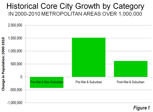
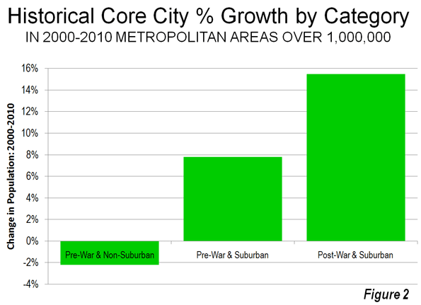
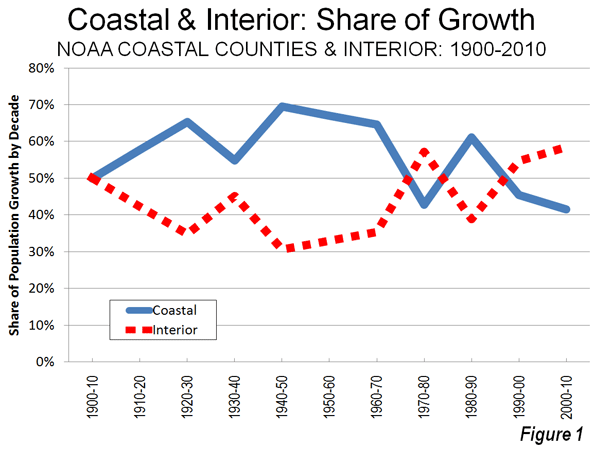
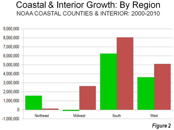
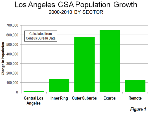
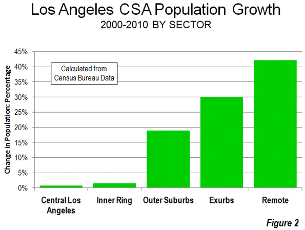
    Growth: 2000 to 2010: The population growth in the Los Angeles CSA was widely dispersed and away from the core. The central area (urban core) of the city Los Angeles extends from the Santa Monica Mountains to South Los Angeles and from the boundaries of Beverly Hills, West Hollywood and Culver City to East Los Angeles grew only 0.7 percent. Uniquely, the central area densified strongly between 1960 and 2000, while other urban cores nearly all declined in population, whether in the United States or Western Europe. Much of this was due to strong immigration from Mexico, other parts of Latin America, as well as Asia.

    The inner suburban ring, which includes the balance of Los Angeles County south of the Santa Susana and San Gabriel Mountains as well as the older northwestern Orange County suburbs grew by 1.5 percent. Within this area, 32 inner suburbs (all in Los Angeles County) grew from 1.766 million to 1.767 million (0.1 percent) from 2000 to 2010 (Note 2).

    The outer suburbs, which include the balance of Orange County (including the Mission Viejo urban area) and the western portions of Riverside and San Bernardino counties (including the Riverside – San Bernardino urban area) grew 19 percent.

    The exurban areas, which include areas outside the core urban areas of Los Angeles, Riverside-San Bernardino and Mission Viejo grew 30 percent. The hot spots included Ventura County, the Santa Clarita Valley, the Antelope Valley, the Victorville-Hesperia area, the Coachella Valley (Indio-Palm Springs), the Hemet area and the Temecula-Murrieta area. An argument could be made that Temecula-Murrieta would be in the San Diego metropolitan area if metropolitan areas were defined by smaller area units, such as municipalities (as in Canada) or census tracts. The exurban areas are more attractive to residents at least in part because of considerably less expensive housing and their greater availability of detached houses than in the three core urban areas.

    More remote areas of the desert extending to the Nevada and Arizona borders added 42 percent to their population (Table 2, Figure 1 and 2).

    Table 2
    Los Angeles CSA: Population by Sector: 2000-2010
    Sector 2000 2010 Change % Change
    Central Los Angeles          1,752,024              1,763,967         11,943 0.7%
    Inner Ring          9,093,756              9,231,513       137,757 1.5%
    Outer Suburbs          3,053,615              3,630,273       576,658 18.9%
    Exurbs          2,173,459              2,822,884       649,425 29.9%
    Remote             301,331                 428,369       127,038 42.2%
    Total       16,374,185            17,877,006    1,502,821 9.2%

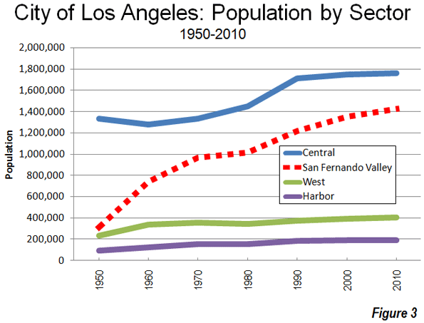
    City of Los Angeles: The dispersion of population was also evident in the city of Los Angeles. For decades, the city of Los Angeles has grown strongly. Approximately one-quarter of this growth since 1960 has been the densifying central area, as noted above.

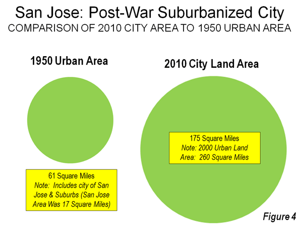
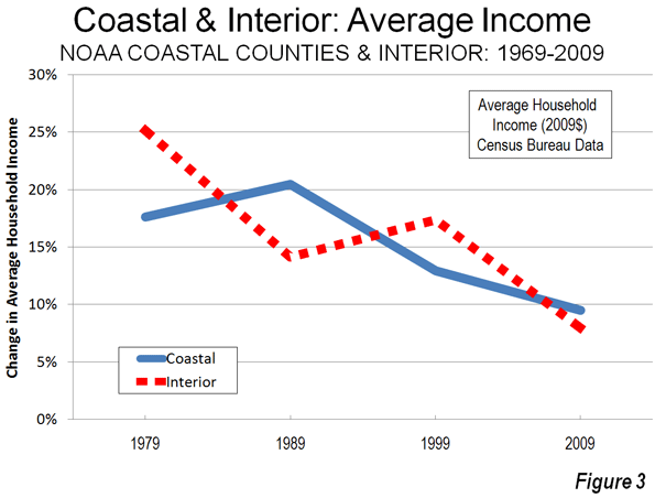
    However, little noted is the fact that most of the city’s growth was greenfield suburban in nature, built at low and moderate densities and largely car-oriented. For most of the past fifty years the growth has been “over the hill” in the San Fernando Valley, a formerly rural area which was annexed by the city before 1930. Between 1950 and 2010, the population of the San Fernando Valley grew from 300,000 to 1,400,000. Thus, the Valley grew like virtually every fast-growing historical core city in the nation that has grown since 1950, by filling up empty land (Figure 3).

    Much has been written about the “Manhattanization” of the Los Angeles core. However, with only 13 towers more than 550 feet, downtown Los Angeles is no threat to Manhattan, with more than 125, or even Chicago with more than 70. Further, job growth is stagnant, with virtually no change in private sector employment over the last decade, despite substantial government subsidies.

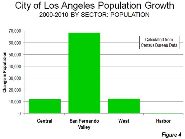
    Between 2000 and 2010, the central area grew at its slowest rate since the 1950s, growing by only 0.7 percent to its population, growing only 12,000 (to 1,764,000) or barely 12 percent of the city’s growth. Nonetheless, and contrary to the reputation of Los Angeles, the central area is very densely populated, at approximately 14,000 people per square mile, with the highest density census tracts having more than 90,000 residents per square mile. Among the nation’s largest municipalities, only New York and San Francisco are denser than central Los Angeles.

    The big story in growth was on periphery. The San Fernando Valley captured 70 percent of the city’s growth in the 2000s, with considerable greenfield expansion in the hills north of Chatsworth and Northridge. Even so, the Valley’s growth was only five percent. The western portion of the city, which extends from the Santa Monica Mountains to Los Angeles International Airport, grew three percent and accounted for 13 percent of the city’s growth. The Harbor area added two percent to its population and accounted for five percent of the city’s growth (Figure 4).

    The Future: Growth or Stagnation? After more than a century of spectacular growth, Los Angeles demographic juggernaut is stagnating and could conceivably go in reverse due to declining immigration, an exodus of middle class and working class families.  Indeed Even the strong growth in the outer suburbs and exurbs was not sufficient to drag the regional population increase (9 percent) up to the national rate of 10 percent between 2000 and 2010.

    The immediate prognosis should be for even slower growth. The financial, regulatory and cost of living disadvantages of California are widely recognized by households and businesses alike. With stronger regulations in the offing, such as the stronger land use restrictions likely to occur as a result of Senate Bill 375, any future growth on the periphery could be dampened. Even with multi-billion support in terms of tax breaks and public investment, the central core seems unlikely to come close to making much of a real difference, at least beyond the media.  Los Angeles may not be on the road to Rust Belt stagnation, but the dynamism of the last century is no more.

    ——

    Note 1: In this article, the term "city" means municipality.

    Note 2: This includes municipalities and census designated places nearest the central area of the city of Los Angeles, from Glendale and Pasadena through Monterey Park to South Gate, Compton and Gardena and to the west of the central area.

    Note 3: Biographical Note: The author was born in the Echo Park district, near downtown Los Angeles.

    Photograph: Downtown Los Angeles from Echo Park (by author)

    Wendell Cox is a Visiting Professor, Conservatoire National des Arts et Metiers, Paris and the author of “War on the Dream: How Anti-Sprawl Policy Threatens the Quality of Life

  • Moving from the Coast

    For years both government and media have been advancing the notion that   America’s coastal counties are obtaining most of the population growth at the expense of interior counties. For example, the National Oceanic and Atmospheric Administration reported in the 1990s: Coastal areas are crowded and becoming more so every day. More than 139 million people–about 53% of the national total–reside along the narrow coastal fringes.

    NOAA went on to say that the population of the coastal counties is expected to increase by an average of 3600 people per day and noted further that the coastal counties were growing faster than the nation as a whole. NOAA has designated 673 counties on four coasts (Atlantic, Gulf, Pacific and Great Lakes) in the contiguous United States, Hawaii and Alaska as coastal counties.

    Population Growth: In fact, coastal counties are not growing faster than the nation as a whole and were not when NOOA issued the 1990s report. For most of the last 40 years, the nation’s interior counties have been adding more population. From 1970 to 2010, interior counties added 55.7 million new residents, compared to 49.7 million new residents in coastal counties. This is a reversal from 1940 to 1970, when two thirds of the nation’s population growth was in the coastal counties.

    The trends today actually have become more favorable for the interior than at any time in a century. From 2000 to 2010, the interior counties captured more of the nation’s growth than in any decade since 1900 (Table). From 2000 to 2010, the interior counties added 16.0 million residents, 59.6 percent of the nation’s growth compared to 11.4 million new residents in the coastal counties.

    Coastal and Interior Population: Counties
    1900-2010
    Coastal Counties Interior Counties United States
    Year Population Share Change Population Share Change Population Change
    1900         30.2 39.7%         46.0 60.3%         76.2
    1910         38.2 41.4%           8.0         54.0 58.6%           8.0         92.2         16.0
    1920         46.2 43.6%           8.0         59.8 56.4%           5.8       106.0         13.8
    1930         57.4 46.6%         11.2         65.8 53.4%           6.0       123.2         17.2
    1940         62.3 47.1%           4.9         69.8 52.9%           4.0       132.2           9.0
    1950         75.2 49.9%         12.9         75.5 50.1%           5.7       150.7         18.5
    1960         94.4 52.6%         19.2         85.0 47.4%           9.5       179.3         28.6
    1970       109.9 54.0%         15.6         93.5 46.0%           8.5       203.4         24.1
    1980       119.8 52.9%           9.9       106.7 47.1%         13.2       226.5         23.2
    1990       133.4 53.6%         13.6       115.3 46.4%           8.6       248.7         22.2
    2000       148.2 52.7%         14.9       133.2 47.3%         17.9       281.4         32.7
    2010       159.6 51.7%         11.4       149.1 48.3%         16.0       308.7         27.3
    Population in Millions
    Calculated from US Census Bureau Data
    Coastal counties designated by NOAA (673 counties)
    Totals may vary due to rounding


    As of 2010, the coastal counties have 51.7 percent of the nation’s population, having dropped from 52.7 percent in 2000 and a peak of 54.0 percent in 1970 (Figure 1). Rather than adding 3600 new people every day, coastal counties added 3100 people per day, while interior counties added 4400 per day during the 2000s. A smaller sample of 559 counties that was examined by economists Jordan Rapaport and Jeffrey Sachs in the early 2000s experienced an even more pronounced movement away from the coasts between 2000 and 2010, with more than 60 percent of the nation’s growth taking place in the interior counties.

    There may also be some concern about density in coastal counties.   Yet Malthusian fears need not grip coastal residents. With a population density of approximately 315 per square mile (120 per square kilometer), the coastal counties of the contiguous United States have only a slightly higher density than the post-enlargement 27-nation European Union. The coastal counties have a density one-half that of Germany. In contrast, the interior counties are far less dense, at 60 persons per square mile.

    There has also been significant change in coastal population trends since the middle 1990s. The largest Pacific Coast metropolitan areas, such as Los Angeles, San Francisco, San Diego, San Jose and Seattle have seen their growth slow considerably. In the 1990s, NOAA was projecting huge population increases for Los Angeles and San Diego counties. It appears likely that these 2015 projections will fall at least 600,000 short in both counties. Even Seattle, arguably the healthiest economically among the west coast metropolitan areas, is now growing more slowly than former laggards Oklahoma City, Indianapolis and Columbus in the interior.

    Regional Population Growth: There was significant variation in growth among the varied regions of the country. In the Northeast, there was much stronger growth on the coast, which added 1.6 million people, compared to a gain of less than 150,000 in the interior. In the Midwest, the coastal counties (along the Great Lakes) lost 120,000 people, while the interior counties gained 2.7 million. In the South, the interior grew more, at 8.1 million, slightly more than 6.3 million in coastal counties.  In the West, interior counties gained 5.1 million people, while the coastal counties gained 3.7 million (Figure 2). This drop in coastal growth was a principal reason why the West grew less quickly than the South, which experienced the most robust coastal growth. For this reason, the West failed to be the nation’s fastest growing region for the first time since 1900.

    Personal Income: Rappaport and Sachs noted in their early 2000s work that the density of economic activity was far greater in the coastal counties. Of course this is to be expected, due to their greater population density. However the data with respect to the distribution of personal income is less clear. Since 1969, coastal and interior counties have been alternating leadership in personal income growth per capita. During the 2000s, interior counties experienced average personal income growth slightly less than that of the coastal counties (Figure 3). However, average per capita income since 1970 has risen 81 percent, compared to a lower 75 percent in the coastal counties (adjusted for inflation).  Overall, the share of income in the interior counties has been growing modestly (Figure 4).

    Domestic Migration: The most important factor in the growth of the interior counties in the 2000s lies with net domestic migration, with more residents moving from the coastal counties to the interior counties. Between 2000 and 2009, 4.5 million people moved to the interior counties, while 4.5 million people moved away from the coastal counties, according to Census Bureau estimates (Figure 5).

    Rappaport and Sachs had theorized that the greater concentration of population and economic activity in the coastal counties could be reflective of a more attractive quality of life. The domestic migration data would suggest that, at least over the last decade, people are opting for the interior, perhaps sensing that the coastal quality of life may not be as affordable and accessible as in the past.  

    Cost of Living: The key here lies with the cost of living, which has become far higher on the coasts then in the interior. The most significant cost of living differences for households are in the cost of housing.   

    From 2000 to 2009, housing affordability deteriorated markedly in the coastal counties. Census Bureau data indicates that the Median Multiple (median house founded divided by median household income) rose from 3.6 to 5.4 in the coastal counties (population weighted). By contrast, housing affordability worsened far less in the interior counties, where the Median Multiple rose from 2.5 to 3.1. Thus, the median household saw owned housing increase 22 months worth of income in value in coastal counties, compared to seven months worth of income in interior counties (Figure 6). At the same time, these higher coastal house prices developed as demand for housing was dropping substantially, with 4.5 million people moving away from coastal counties (above).

    Many of the coastal counties have strong land use regulation (smart growth or urban containment regulation), especially in California, Oregon, Washington, Florida and the metropolitan areas of Boston, New York and Washington. A considerable body of research, both econometric and descriptive, has associated more restrictive land use regulation (called smart growth, urban consolidation or urban containment) with higher house price increases, reaching back at least to the seminal 1970s work by Sir Peter Hall and his associates in the United Kingdom. It thus seems likely that the deterioration of housing affordability in coastal counties is materially associated with their less robust growth. The quality of life on the coasts may simply have become too expensive.

    The Future? It is unclear whether the recent higher population growth rates, stronger migration trends and improved economic performance of the interior will continue into the future. The 1940 to 1970 dominance of the coastal counties surged as coastal metropolitan areas, especially in Florida and California, grew much more quickly. Now that pattern has been reversed.  More favorable trends over the past 40 years in the interior counties seem likely continue, unless coastal house prices and the cost of living begin to swing back toward the national norm.

    —-

    Note: Complete county data is at County Coastal Population (also attached to this article)

    Photograph: San Diego, which experienced greater domestic outmigration than Pittsburgh in the 2000s.

  • Land Use Regulation Blamed for High Hong Kong House Prices

    The Wall Street Journal  reports that growing concern about Hong Kong’s high house prices has led the special administrative region’s Chief Executive Donald Tsang to promise an overhaul of housing and land use policies in the fall.     

    Chou Hong-Wing, a real estate professor at Hong Kong University told The Wall Street Journal  that "Hong Kong isn’t short of land." Chief Executive Tsang indicated agreement, saying that the only way to solve the problem in the long run is tackling "market demand and land supply."

    A broad array of economic research has documented the higher house prices that occur where there land supply is overly restricted. In a survey of seven nations, Hong Kong was rated as the most unaffordable market in the 7th Annual Demographia Housing Affordability Survey in January, with a Median Multiple of 11.4 (median house price divided by median household income). Sydney and Vancouver, both with stringent land rationing (smart growth) programs ranked second and third, at 9.6 and 9.5 respectively.