Category: Demographics

Is There A Civilization War Going On?

“Civilizations die from suicide, not by murder.” — Arnold J. Toynbee

From the heart of Europe to North America, nativism, sometimes tinged by white nationalist extremism, is on the rise. In recent elections, parties identified, sometimes correctly, as alt-right have made serious gains in Germany, Austria and the Czech Republic, pushing even centrist parties in their direction. The election of Donald Trump can also be part of this movement.

Why is this occurring? There are economic causes to be sure, but perhaps the best explanation is cultural, reflecting a sense, not totally incorrect, that western civilization is on the decline, a movement as much self-inflicted as put upon.

French intellectuals first to see the trend

In 1973 a cranky French intellectual, Jean Raspail, published a speculative novel, “The Camp of the Saints,” which depicted a Europe overrun by refugees from the developing world. In 2015 another cranky Frenchman, Michael Houellenbecq, wrote a bestseller, “Submission,” which predicted much the same thing, ending with the installation of an Islamist government in France.

Both novels place the blame for the collapse of the Western liberal state not on the immigrants but on cultural, political and business leaders all too reluctant to stand up for their own civilization. This is reflected in such things as declining respect for free speech, the importance of citizenship, and even the weakening of the family, an institution now rejected as bad for the environment and even less enlightened than singlehood.

Critically, the assault on traditional liberalism has come mostly not from the reactionary bestiary, but elements of the often-cossetted left. It is not rightist fascism that threatens most but its pre-condition, the systematic undermining of liberal society from within.

Read the entire piece at The Orange County Register.

Joel Kotkin is executive editor of NewGeography.com. He is the Roger Hobbs Distinguished Fellow in Urban Studies at Chapman University and executive director of the Houston-based Center for Opportunity Urbanism. His newest book is The Human City: Urbanism for the rest of us. He is also author of The New Class Conflict, The City: A Global History, and The Next Hundred Million: America in 2050. He lives in Orange County, CA.

Photo: JÄNNICK Jérémy [CC BY 3.0], via Wikimedia Commons

October 30, 2017

Highest Cost Rental Markets: Even Worse for Buyers

There is considerable concern about rising rents, especially in the most expensive US housing markets. Yet as tough as rising rents are, the high rent markets are also plagued by even higher house costs relative to the rest of the nation. As a result, progressing from renting to buying is all the more difficult in these areas.

This is illustrated by American Community Survey data for the nation’s 53 major housing markets (metropolitan areas with more than 1,000,000 residents). The range in median contract rent between the major housing markets 3.1 times, with San Jose being the most expensive and Rochester the least. The range in median house values was more than double that, at 6.6 times, between highest cost San Jose and lowest cost Pittsburgh. Thus, house prices in the most expensive markets tend to be far higher in relation to rents than in the less expensive markets.

The rising difference between house values and rents was noted last year in The House Prices are Too Damned High, which showed that from 1969 to 2015, the difference in the range between rentals and house values rose from 51 percentage points to 375 percentage points (Figure 1). It is no coincidence that 1969 was the last census data before far more strict land use regulations were implemented in some major housing markets.

The House Value-to-Rent Ratio

This is illustrated by the median house value-to-rent ratio, which is calculated by dividing the median house value by the median contract rent per year (monthly times 12). Overall in 2016, the median contract rent was $841 in the United States, while the median house value was $205,000. This calculates to a value-to-rent ratio of 20.3.

Where Housing Aspiration is Most Challenging

California, long home to house prices far above the rest of the nation dominates the list of housing markets in which it is hardest for buyers to move up to home ownership. The worst market is the San Francisco metropolitan area, where the median house value in 2016 was nearly 40 times the median annual rent (39.6) and nearly twice the national figure of 20.3. San Jose is the second worst market, with a value-to-rent ratio of 38.7. Los Angeles is third where the median house value is 36.9 times the median annual rent. There is a larger gap down to San Diego, ranked fourth worst, where there is a median value-to-rent ratio of 31.1. Sacramento is also in the least friendly five for renters aspiring to be buyers, with a value-to-rent ratio of 29.6. This may be a surprising finding and is discussed further below. California’s other major market, Riverside-San Bernardino does better, ranking 13th worst, with a value-to-rent ratio of 24.5.

Even with New York’s notoriously high rents, it did not muscle out California in the worst five. New York’s s value-to-rent ratio was 29.5 The balance of the 10 markets in which moving from renting to buying is most difficult also includes #7 Boston (28.1), #8 Portland (27.9), #9 Providence (27.7) and #10 Seattle (27.2).

Comparison with Demographia Housing Affordability Ratings

The eleven housing markets with the highest value-to-rent ratios have ratings of “severely unaffordable” in the 13th Annual Demographia International Housing Affordability Survey. This is the least affordable rating (Figure 2) and indicates a median multiple of 5.1 or higher (median house price divided by median household income). The 12th highest value-to-rent ratio is in Salt Lake City, which is rated “seriously unaffordable,” the second most unaffordable category. Thirteenth ranked Riverside-San Bernardino was the only other severely unaffordable major U.S. housing market in the Demographia survey.

Each of the severely unaffordable markets have land use restrictions that make it virtually impossible to build the low-cost suburban tract housing crucial to retaining housing affordability. In such markets, Buildzoon.coms’ economist Issi Romem has shown that house values have become detached from construction costs, largely the result of rising land prices (which are associated with stronger land use regulation, especially urban containment policy).

The Surprising Case of Sacramento

Sacramento’s high cost housing may come as a surprise. Sacramento has often “slipped under the radar” as a severely unaffordable market, yet was so from 2004 through 2008.Sacramento had reached a median multiple of 6.8 in 2005 before the housing bust and was less affordable than Vancouver, the third least affordable housing market out of nine nations rated in 2016 by Demographia. Sacramento again became severely unaffordable in last year’s Demographia survey reaching a median multiple of 5.1. But there is reason for concern in Sacramento, which has seen its median multiple rise from 2.9 to 5.1 in just four years. Any continuation of such this trend could result in a material deterioration of Sacramento’s value-to-rent ratio, made all the more likely by California’s overly restricted housing and land use regulations.

The Value-to-Rent Ratio and Inequality

Rising inequality is a widespread concern. Yet, as researchers have shown, much of the expanding inequality is centered in the value of owned housing, which has been associated with more restrictive land and housing regulation. In the United States, the price is being paid for by younger households, who are faced with greater student loan debts and a less lucrative economy. It is also paid for by ethnic minority households, whose more limited incomes are making the jump to home ownership even more difficult (See: Progressive Cities: Home of the Worst Housing Inequality).

Median House Value to Median Contract Rent Ratios
53 Major US Housing Markets (Metropolitan Areas)
Worst Markets for Moving from Renting to Buying
Rank	Housing Market (Metropolitan Area)	Value-to-Rent Ratio	Median Contract Rent (Monthly)	Median House Value	Housing Affordabilty Rating
1	San Francisco-Oakland, CA	39.56	$1,677	$796,100	Severely Unaffordable
2	San Jose, CA	38.69	$1,964	$911,900	Severely Unaffordable
3	Los Angeles, CA	36.92	$1,305	$578,200	Severely Unaffordable
4	San Diego, CA	31.07	$1,415	$527,600	Severely Unaffordable
5	Sacramento, CA	29.62	$1,022	$363,300	Severely Unaffordable
6	New York, NY-NJ-PA	29.05	$1,223	$426,300	Severely Unaffordable
7	Boston, MA-NH	28.14	$1,222	$412,700	Severely Unaffordable
8	Portland, OR-WA	27.89	$1,031	$345,000	Severely Unaffordable
9	Providence, RI-MA	27.77	$796	$265,300	Seriously Unaffordable
10	Seattle, WA	27.23	$1,198	$391,500	Severely Unaffordable
11	Denver, CO	24.79	$1,174	$349,200	Severely Unaffordable
12	Salt Lake City, UT	24.60	$907	$267,800	Moderately Unaffordable
13	Riverside-San Bernardino, CA	24.47	$1,086	$318,900	Severely Unaffordable
14	Washington, DC-VA-MD-WV	23.74	$1,444	$411,400	Seriously Unaffordable
15	Baltimore, MD	23.21	$1,055	$293,900	Moderately Unaffordable
16	Milwaukee,WI	23.07	$737	$204,000	Seriously Unaffordable
17	Hartford, CT	22.83	$903	$247,400	Moderately Unaffordable
18	Raleigh, NC	22.56	$878	$237,700	Moderately Unaffordable
19	Philadelphia, PA-NJ-DE-MD	22.27	$919	$245,600	Moderately Unaffordable
20	Las Vegas, NV	22.06	$883	$233,700	Seriously Unaffordable
21	Phoenix, AZ	21.97	$876	$231,000	Seriously Unaffordable
22	Richmond, VA	21.81	$868	$227,200	Moderately Unaffordable
23	Minneapolis-St. Paul, MN-WI	21.64	$926	$240,500	Moderately Unaffordable
24	Virginia Beach-Norfolk, VA-NC	21.27	$940	$239,900	Moderately Unaffordable
25	Austin, TX	21.20	$1,035	$263,300	Seriously Unaffordable
26	Cincinnati, OH-KY-IN	21.08	$653	$165,200	Affordable
27	Nashville, TN	21.00	$829	$208,900	Moderately Unaffordable
28	Louisville, KY-IN	20.94	$645	$162,100	Moderately Unaffordable
29	St. Louis,, MO-IL	20.64	$683	$169,200	Affordable
30	Chicago, IL-IN-WI	20.60	$930	$229,900	Moderately Unaffordable
31	Kansas City, MO-KS	20.38	$711	$173,900	Affordable
32	Columbus, OH	20.15	$712	$172,200	Affordable
33	Birmingham, AL	20.15	$637	$154,000	Moderately Unaffordable
34	New Orleans. LA	19.89	$788	$188,100	Moderately Unaffordable
35	Oklahoma City, OK	19.86	$647	$154,200	Affordable
36	Tucson, AZ	19.82	$716	$170,300	Moderately Unaffordable
37	Charlotte, NC-SC	19.77	$793	$188,100	Moderately Unaffordable
38	Pittsburgh, PA	19.62	$631	$148,600	Affordable
39	Miami, FL	19.36	$1,122	$260,600	Severely Unaffordable
40	Grand Rapids, MI	19.20	$714	$164,500	Affordable
41	Atlanta, GA	18.72	$880	$197,700	Moderately Unaffordable
42	Buffalo, NY	18.63	$636	$142,200	Affordable
43	Cleveland, OH	18.47	$659	$146,100	Affordable
44	Indianapolis. IN	18.43	$694	$153,500	Affordable
45	Detroit, MI	18.37	$729	$160,700	Affordable
46	Jacksonville, FL	18.33	$853	$187,600	Moderately Unaffordable
47	Dallas-Fort Worth, TX	18.13	$869	$189,100	Moderately Unaffordable
48	Orlando, FL	17.72	$948	$201,600	Seriously Unaffordable
49	Memphis, TN-MS-AR	17.69	$671	$142,400	Moderately Unaffordable
50	Houston, TX	17.36	$871	$181,400	Moderately Unaffordable
51	San Antonio, TX	16.65	$802	$160,200	Moderately Unaffordable
52	Tampa-St. Petersburg, FL	16.61	$879	$175,200	Seriously Unaffordable
53	Rochester, NY	15.97	$725	$138,900	Affordable

Sources: American Community Survey 2016, 13th Annual Demographia International Housing Affordability Survey.

Wendell Cox is principal of Demographia, an international public policy and demographics firm. He is a Senior Fellow of the Center for Opportunity Urbanism (US), Senior Fellow for Housing Affordability and Municipal Policy for the Frontier Centre for Public Policy (Canada), and a member of the Board of Advisors of the Center for Demographics and Policy at Chapman University (California). He is co-author of the “Demographia International Housing Affordability Survey” and author of “Demographia World Urban Areas” and “War on the Dream: How Anti-Sprawl Policy Threatens the Quality of Life.” He was appointed to three terms on the Los Angeles County Transportation Commission, where he served with the leading city and county leadership as the only non-elected member. He served as a visiting professor at the Conservatoire National des Arts et Metiers, a national university in Paris.

Photograph: Sacramento – One of 5 most difficult markets for moving from renting to buying.

October 27, 2017

Superstar Effect: Venture Capital Investments

This is the latest in my “superstar effect” series. Richard Florida posted an interesting analysis of venture capital investments over at City Lab.

Four cities dominate the charts: San Francisco Bay Area, New York, Boston, and Southern California. Call them the Big Four. No place else is even close.

It’s not just that they dominate in total dollars as in the above graph. They also dominate in total number of deals, with 52% of the national total. So it’s not just a handful of big deals making the Big Four standout.

Florida points out that the data don’t back up the idea of the rise of the rest. The superstars account remain in a league apart as far as VC investment goes.

That doesn’t mean the interior is getting nothing. Certainly plenty of cities now have tech startups where there were none before. That’s reason to celebrate. But it’s too early to declare a major decentralization of VC activity.

Also, tech has historically been a very cyclical industry. The last crash wiped out almost all emerging startup clusters – even New York’s Silicon Alley. We’ll have to see how things shake out in the next crash when it comes.

In the meantime, there remains a superstar bias in VC funding.

This piece originally appeared on Urbanophile.

Aaron M. Renn is a senior fellow at the Manhattan Institute, a contributing editor of City Journal, and an economic development columnist for Governing magazine. He focuses on ways to help America’s cities thrive in an ever more complex, competitive, globalized, and diverse twenty-first century. During Renn’s 15-year career in management and technology consulting, he was a partner at Accenture and held several technology strategy roles and directed multimillion-dollar global technology implementations. He has contributed to The Guardian, Forbes.com, and numerous other publications. Renn holds a B.S. from Indiana University, where he coauthored an early social-networking platform in 1991.

Photo: Vik Waters [CC BY-SA 2.0], via Wikimedia Commons

October 18, 2017
Ending Economic Apartheid

Thanks to its greenbelt and slow-growth policies, Boulder, Colorado is the nation’s most-expensive and least-affordable housing market of any city not in a coastal state. As a result, as noted in an op-ed in The Hill, the number of black residents in Boulder declined by 30 percent between 2010 and 2016, leaving less than 1.6 percent of the city with African-American ancestry.

Closer to my home, the Bend Bulletin argues that the state of Oregon “works against affordable housing by, among other things. . . artificially increas[ing] the price of land through its urban growth boundary system.” Although cities are required to maintain an inventory of developable land within their growth boundaries, the paper notes that permission to expand their boundaries takes years.

The Oregon legislature effectively admitted that this is a problem last year when it passed a law allowing two cities to develop land on up to 50 acres of land outside of their growth boundaries. But can anyone seriously believe that adding 100 acres of new housing will make housing more affordable in Oregon?

To make matters worse, the law is to be administered by the state Land Conservation and Development Commission, the same commission that wrote the rules requiring urban-growth boundaries in the first place. Even if 100 acres were enough, they certainly won’t be timely. Applications to be one of the pilot cities are due November 1, more than a year after the law is passed. Considering this is actually only a preapplication, it could take another year to get final approval. Once approved, the pilot cities will probably take a year or more to implement their plans. Those plans will no doubt be appealed by 1000 Friends of Oregon or some other group. So it may be several years in all before ground is broken for the first new home under this law.

This is the wrong way of dealing with land use in general and housing affordability in particular. Oregon needs to abandon urban-growth boundaries and Boulder needs to abandon its greenbelt and its limit on construction permits. These policies violate people’s property rights and freedom of movement. In the end, it will probably take a court ruling, not a legislative action, to strike them down.

This piece first appeared on The Antiplanner.

Randal O’Toole is a senior fellow with the Cato Institute specializing in land use and transportation policy. He has written several books demonstrating the futility of government planning. Prior to working for Cato, he taught environmental economics at Yale, UC Berkeley, and Utah State University.

Photo: Eddyl [CC BY-SA 3.0], via Wikimedia Commons

October 17, 2017
What Does the Future Hold for the Automobile?

For a generation, the car has been reviled by city planners, greens and not too few commuters. In the past decade, some boldly predicted the onset of “peak car” and an auto-free future which would be dominated by new developments built around transit.

Yet “peak car,” like the linked concept of “peak oil” has failed to materialize. Once the economy began to recover from the Great Recession, vehicle miles traveled, sales of cars, and particularly trucks, began to rise again, reaching a sales peak the last two year. Instead, it has been transit ridership that has stagnated, and even fallen in some places like Southern California.

Demographics — notably the rise of the millennial generation — were once seen as the key to unlocking a post-car future. Yes, younger people have been slower to buy cars than their predecessors, much as they have been slow to get full-time jobs, marry or buy homes, but more are now driving, so to speak, the car market, representing the largest share of new automobile buyers.

Convenience can’t be banned

The persistence of personal transportation has little to do with the much hyped “love affair” with the automobile but convenience and access to work. Simply put, with a few notable exceptions, Americans live in increasingly “dispersed regions.” Transit works brilliantly, as Wendell Cox and I demonstrated recently in a paper for Chapman’s Center for Demographics, to downtown San Francisco and a few other “legacy” urban centers, notably New York which accounts for a remarkable 40 percent of all transit commuting in the United States.

Yet, overall, 90 percent of Americans get to work in cars. Access to jobs represents a key factor. University of Minnesota research shows that the average employee in 49 of the nation’s 52 major metropolitan areas can reach barely 1 percent of the jobs in the area by transit within 30 minutes while cars offer upwards of 70 times more access. This practical concern does much to explain why up to 76 percent of all work trips remain people driving alone.

Read the entire piece at The Orange County Register.

Joel Kotkin is executive editor of NewGeography.com. He is the Roger Hobbs Distinguished Fellow in Urban Studies at Chapman University and executive director of the Houston-based Center for Opportunity Urbanism. His newest book is The Human City: Urbanism for the rest of us. He is also author of The New Class Conflict, The City: A Global History, and The Next Hundred Million: America in 2050. He lives in Orange County, CA.

Photo: Nissan_LEAF_got_thirsty.jpg: evgonetwork (eVgo Network). Original image was trimmed and retouched (lighting and color tones) by User:Mariordoderivative work: Mariordo [CC BY 2.0], via Wikimedia Commons

October 16, 2017

Progressive Cities: Home of the Worst Housing Inequality

America’s most highly regulated housing markets are also reliably the most progressive in their political attitudes. Yet in terms of gaining an opportunity to own a house, the price impacts of the tough regulation mean profound inequality for the most disadvantaged large ethnicities, African-Americans and Hispanics.

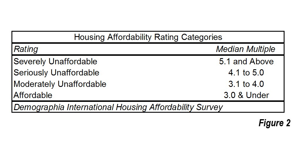
Based on the housing affordability categories used in the Demographia International Housing Affordability Survey for 2016 (Table 1), housing inequality by ethnicity is the worst among the metropolitan areas rated “severely unaffordable.” In these 11 major metropolitan area markets, the most highly regulated, median multiples (median house price divided by median household income) exceed 5.0. For African-Americans, the median priced house is 10.2 times median incomes. This is 3.7 more years of additional income than the overall average in these severely unaffordable markets, where median house prices are 6.5 times median household incomes. It is only marginally better for Hispanics, with the median price house at 8.9 times median household incomes, 2.4 years more than the average in these markets (Figure 1).

The comparisons with the 13 affordable markets (median multiples of 3.0 and less) is even more stark. For African-American households things are much better than in the more progressive and most expensive metropolitan areas. The median house prices is equal to 4.6 years of median income, 5.5 years less than in the severely affordable markets. Moreover, for African-Americans, housing affordability is only marginally worse than the national average in the affordable market.

Things are even better for Hispanics, who would find the median house price 3.8 times median incomes, 5.1 years less than in the severely affordable markets. This is better than the national average housing affordability.

Among the four markets rated “seriously unaffordable,” (median multiple from 4.1 to 5.0) the inequality is slightly less, with African-Americans finding median house prices equal to 2.2 years of additional income compared to average. The disadvantage for Hispanics is 1.5 years.

In contrast, inequality is significantly reduced in the less costly “moderately unaffordable” markets (median multiple of 3.1 to 4.0) and the “affordable” markets (median multiple of 3.0 and less).

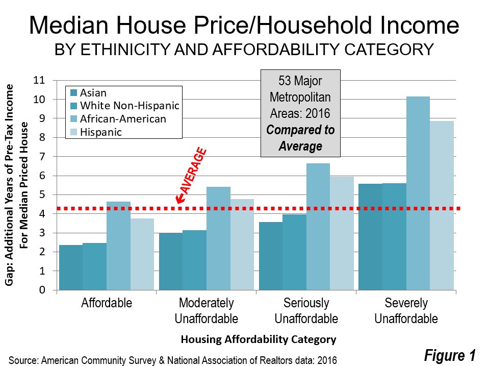
The discussion below describes the 10 largest and smallest housing affordability gaps for African-American and Hispanic households relative to the average household, within the particular metropolitan markets. The gaps within ethnicities compared to the affordable markets would be even more. The four charts all have the same scale (a top housing affordability gap of 10 years) for easy comparison.

able 2 illustrates housing affordability gaps by major metropolitan areas. There are also housing affordability ranking gap tables by African-American households (Table 3) and Hispanic households (Table 4).

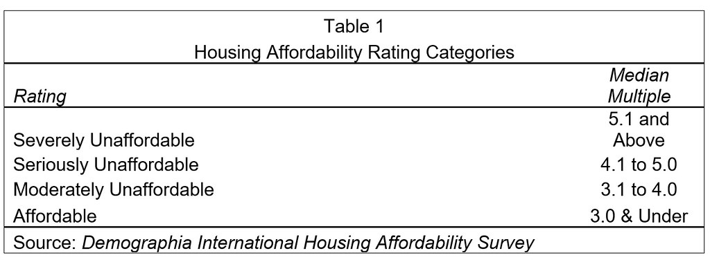
Largest Housing Affordability Gaps: African American

African-Americans have the largest housing affordability inequality gap. And these gaps are most evident in some of the nation’s most progressive cities. The largest gap is in San Francisco, where the median income African-American household faces median house prices that are 9.3 years of income more than the average. In nearby San Jose ranks the second worst, where the gap is 6.2 years. Overall, the San Francisco Bay Area suffers by far the area of least housing affordability for African-Americans compared to the average household.

Portland, long the darling of the international urban planning community, ranks third worst, where the median income African-American household to purchase the median priced house. Milwaukee and Minneapolis – St. Paul ranked fourth and fifth worst followed by Boston, Seattle, Los Angeles, Sacramento and Chicago (Figure 2).

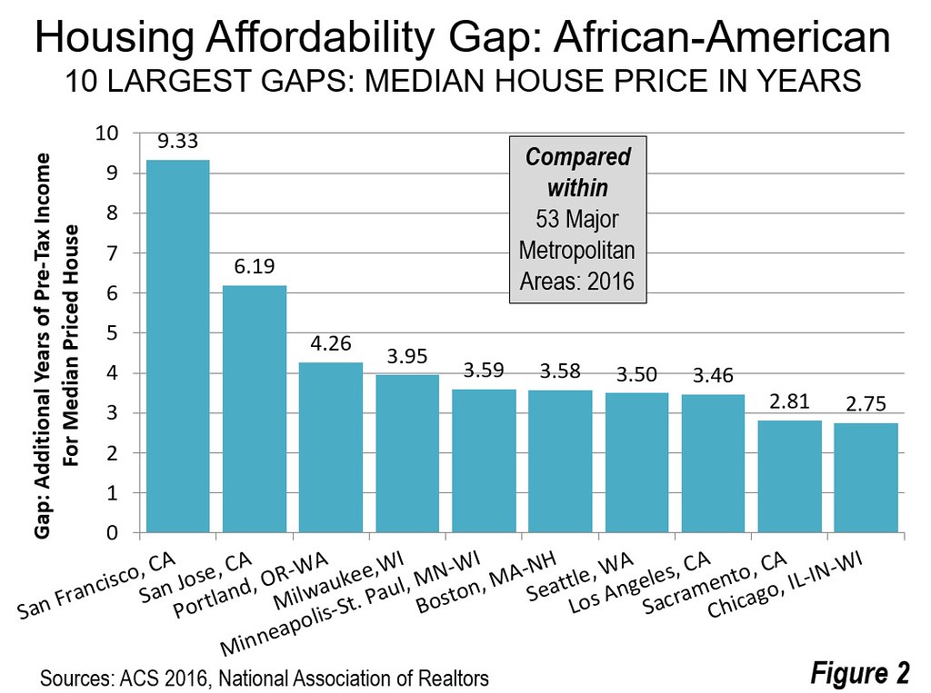
Largest Housing Affordability Gaps: Hispanics

Two of the three worst positions are occupied by the two metropolitan areas in the San Francisco Bay Area. The worst housing affordability gap for Hispanics is in San Jose, a more than one-quarter Hispanic metropolitan area where the median income Hispanic household would require 5.0 years of additional income to pay for the median priced house compared to the average. Boston ranks second worst at 3.9. San Francisco third worst at 3.3 years. Providence and New York rank fourth and fifth worst. The second five worst housing inequality for Hispanics is in San Diego, Hartford, Rochester, Philadelphia and Raleigh (Figure 3).

The San Francisco Bay Area: “Inequality City”

Perhaps no part of the country is more renowned for its progressive politics and politicians than the San Francisco Bay Area. Yet, in housing equality, the Bay Area is anything but progressive. If the African-American and Hispanic housing inequality measures are averaged, disadvantaged minorities face house prices that average approximately 6.25 years more years of median income in San Francisco and 5.60 more years of median income in San Jose.

Moreover, no one should imagine that recent state law authorizing a $4 billion “affordable housing” bond election will have any significant impact. According to the Sacramento Bee, voter approval would lead to 70,000 new housing units annually, when the need for low and very low income households is 1.5 million. The bond issue would do virtually nothing for the many middle-income households who are struggling to pay the insanely high housing costs California’s regulatory nightmare has developed.

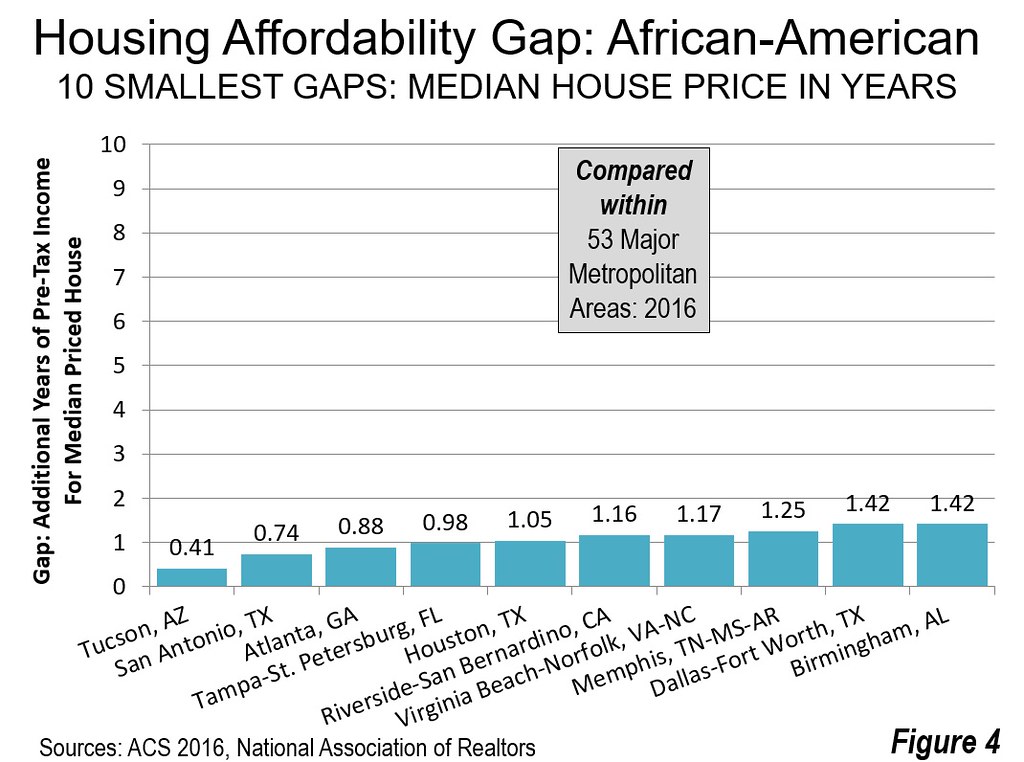
Smallest Housing Affordability Gaps: African-American

Tucson has the smallest housing affordability gap for African-Americans. In Tucson, the median income African-American household would pay approximately 0.4 years (four months) more in income for the median priced house than the average household. In San Antonio, Atlanta and Tampa – St. Petersburg, the housing affordability gaps are under 1.0. Houston, Riverside – San Bernardino, Virginia Beach – Norfolk, Memphis, Dallas – Fort Worth and Birmingham round out the second five. It may be surprising that eight of the metropolitan areas with the smallest housing affordability gaps for African-Americans are in the South and perhaps most surprisingly of all that one of the best, at number 10, is Birmingham. (Figure 4).

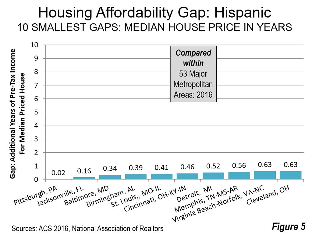
Smallest Housing Affordability Gaps: Hispanic

Among Hispanic households, the smallest housing affordability gap is in Pittsburgh, where the median priced house would require less than 10 days more in median income for a Hispanic household compared the overall average. In Jacksonville the housing affordability gap for Hispanics would be less than two months. In Baltimore, Birmingham, St. Louis and Cincinnati, the median house price is the equivalent of less than six months of median income for an Hispanic household. Detroit, Memphis, Virginia Beach – Norfolk and Cleveland round out the ten smallest housing affordability gaps for Hispanics (Figure 5).

Housing Affordability is the Best for Asians

Recent American Community Survey data indicated that Asians have median household incomes a quarter above those of White Non-– Hispanics. This advantage is also illustrated in the housing affordability data. Asians have better housing affordability than White Non-– Hispanics in 37 of the 53 major metropolitan areas (over 1 million population).

The Importance of Housing Opportunity

Housing opportunity is important. African-Americans and Hispanics already face challenges given their generally lower incomes. However, by no serious political philosophy, progressive or otherwise, should any ethnicity find themselves even further disadvantaged by political barriers, such as have been created by over-zealous land and housing regulators.

Table 2
Housing Affordability Gap by Ethnicity: 2016
53 Major Metropolitan Areas (Over 1,000,000 Population)
Median Multiple (Median house price divided by median household income)

MSA	Median Multiple: All Households	Median Multiple: African-American	African American Housing Affordability Gap in Years	Ranked Most to Least Equal: African-American	Median Multiple: Hispanic	Hispanic Housing Affordability Gap in Years	Ranked Most to Least Equal: Hispanic	Exhibit: Median Multiple: Asian	Exhibit: Median Multiple: White Non-Hispanic

Atlanta, GA	2.95	3.83	0.88	3	3.65	0.70	13	2.30	2.45
Austin, TX	4.00	5.69	1.69	19	5.04	1.04	24	3.23	3.52
Baltimore, MD	3.29	4.75	1.46	12	3.64	0.34	3	2.60	2.83
Birmingham, AL	3.57	4.99	1.42	10	3.96	0.39	4	2.95	3.02
Boston, MA-NH	5.11	8.69	3.58	47	9.02	3.90	52	4.67	4.62
Buffalo, NY	2.48	4.79	2.32	38	4.58	2.10	43	2.90	2.20
Charlotte, NC-SC	3.47	4.95	1.47	13	4.77	1.30	32	2.31	3.08
Chicago, IL-IN-WI	3.56	6.30	2.75	43	4.45	0.90	20	2.69	2.94
Cincinnati, OH-KY-IN	2.53	4.70	2.17	35	2.99	0.46	6	1.75	2.33
Cleveland, OH	2.54	4.50	1.96	27	3.17	0.63	10	1.49	2.16
Columbus, OH	2.91	4.78	1.87	24	4.10	1.19	30	2.50	2.68
Dallas-Fort Worth, TX	3.56	4.98	1.42	9	4.70	1.14	26	2.55	2.87
Denver, CO	5.34	7.64	2.29	37	7.40	2.05	42	5.33	4.76
Detroit, MI	4.01	6.71	2.70	41	4.53	0.52	7	2.56	3.48
Grand Rapids, MI	2.68	4.66	1.98	28	3.85	1.16	28	2.95	2.53
Hartford, CT	3.18	4.88	1.70	20	5.48	2.29	47	2.78	2.82
Houston, TX	3.52	4.57	1.05	5	4.68	1.15	27	2.54	2.65
Indianapolis. IN	2.82	4.89	2.07	31	4.45	1.63	38	2.48	2.50
Jacksonville, FL	3.71	5.15	1.43	11	3.88	0.16	2	3.32	3.38
Kansas City, MO-KS	2.95	4.96	2.00	30	3.97	1.02	23	2.64	2.68
Las Vegas, NV	4.37	6.36	1.98	29	5.19	0.82	16	3.63	3.85
Los Angeles, CA	7.69	11.15	3.46	45	9.74	2.05	41	6.68	6.03
Louisville, KY-IN	2.99	4.90	1.91	25	3.92	0.93	21	2.48	2.71
Memphis, TN-MS-AR	3.12	4.37	1.25	8	3.68	0.56	8	2.13	2.29
Miami, FL	5.94	7.58	1.64	17	6.64	0.70	12	4.39	4.68
Milwaukee,WI	3.93	7.88	3.95	49	5.79	1.86	40	2.78	3.33
Minneapolis-St. Paul, MN-WI	3.24	6.83	3.59	48	4.64	1.40	34	3.25	3.01
Nashville, TN	3.74	5.43	1.69	18	5.04	1.30	33	3.12	3.43
New Orleans. LA	3.85	6.42	2.57	40	5.02	1.17	29	4.01	2.93
New York, NY-NJ-PA	5.40	7.85	2.45	39	8.22	2.82	49	4.68	4.25
Oklahoma City, OK	2.74	4.81	2.07	32	3.62	0.88	19	2.52	2.45
Orlando, FL	4.28	6.00	1.72	22	5.21	0.94	22	2.93	3.60
Philadelphia, PA-NJ-DE-MD	3.42	5.69	2.28	36	5.59	2.17	45	3.02	2.82
Phoenix, AZ	4.01	5.54	1.53	14	5.07	1.06	25	3.17	3.62
Pittsburgh, PA	2.68	4.61	1.93	26	2.70	0.02	1	1.97	2.54
Portland, OR-WA	5.11	9.38	4.26	50	6.69	1.57	37	4.44	4.89
Providence, RI-MA	4.26	6.38	2.12	34	7.21	2.95	50	3.09	3.95
Raleigh, NC	3.46	5.01	1.56	15	5.59	2.13	44	2.47	3.12
Richmond, VA	3.74	5.44	1.70	21	4.61	0.87	18	2.75	3.14
Riverside-San Bernardino, CA	5.38	6.55	1.16	6	6.04	0.66	11	4.04	4.85
Rochester, NY	2.42	4.52	2.10	33	4.67	2.25	46	2.26	2.21
Sacramento, CA	5.00	7.81	2.81	44	6.21	1.21	31	4.63	4.46
St. Louis,, MO-IL	2.74	4.46	1.72	23	3.15	0.41	5	2.41	2.45
Salt Lake City, UT	4.00		No data		5.49	1.49	36	3.70	3.77
San Antonio, TX	3.69	4.43	0.74	2	4.41	0.72	15	2.89	2.86
San Diego, CA	7.98	10.72	2.74	42	10.65	2.67	48	6.88	6.94
San Francisco-Oakland, CA	8.67	18.01	9.33	52	11.93	3.26	51	7.96	7.29
San Jose, CA	9.09	15.28	6.19	51	14.08	5.00	53	7.80	8.24
Seattle, WA	5.27	8.77	3.50	46	7.02	1.74	39	4.55	5.00
Tampa-St. Petersburg, FL	3.87	4.86	0.98	4	4.74	0.87	17	2.85	3.65
Tucson, AZ	4.00	4.41	0.41	1	4.71	0.71	14	4.17	3.54
Virginia Beach-Norfolk, VA-NC	3.48	4.65	1.17	7	4.11	0.63	9	2.94	3.00
Washington, DC-VA-MD-WV	4.08	5.64	1.57	16	5.54	1.46	35	3.76	3.38

Overall median multiple from Demographia International Housing Affordability Survey: Updated with revised income data from 2016 ACS.
Median multiple: Median house price divided by median household income


Table 3
African-American Housing Affordability Gap Ranked: Most to Least Equal
53 Major Metropolitan Areas (Over 1,000,000 Population)
Median Multiple (Median house price divided by median household income)

MSA	Median Multiple: All Households	Median Multiple: African-American	African American Housing Affordability Gap in Years	Ranked Most to Least Equal: African-American	Median Multiple: Hispanic	Hispanic Housing Affordability Gap in Years	Ranked Most to Least Equal: Hispanic	Exhibit: Median Multiple: Asian	Exhibit: Median Multiple: White Non-Hispanic

Tucson, AZ	4.00	4.41	0.41	1	4.71	0.71	14	4.17	3.54
San Antonio, TX	3.69	4.43	0.74	2	4.41	0.72	15	2.89	2.86
Atlanta, GA	2.95	3.83	0.88	3	3.65	0.70	13	2.30	2.45
Tampa-St. Petersburg, FL	3.87	4.86	0.98	4	4.74	0.87	17	2.85	3.65
Houston, TX	3.52	4.57	1.05	5	4.68	1.15	27	2.54	2.65
Riverside-San Bernardino, CA	5.38	6.55	1.16	6	6.04	0.66	11	4.04	4.85
Virginia Beach-Norfolk, VA-NC	3.48	4.65	1.17	7	4.11	0.63	9	2.94	3.00
Memphis, TN-MS-AR	3.12	4.37	1.25	8	3.68	0.56	8	2.13	2.29
Dallas-Fort Worth, TX	3.56	4.98	1.42	9	4.70	1.14	26	2.55	2.87
Birmingham, AL	3.57	4.99	1.42	10	3.96	0.39	4	2.95	3.02
Jacksonville, FL	3.71	5.15	1.43	11	3.88	0.16	2	3.32	3.38
Baltimore, MD	3.29	4.75	1.46	12	3.64	0.34	3	2.60	2.83
Charlotte, NC-SC	3.47	4.95	1.47	13	4.77	1.30	32	2.31	3.08
Phoenix, AZ	4.01	5.54	1.53	14	5.07	1.06	25	3.17	3.62
Raleigh, NC	3.46	5.01	1.56	15	5.59	2.13	44	2.47	3.12
Washington, DC-VA-MD-WV	4.08	5.64	1.57	16	5.54	1.46	35	3.76	3.38
Miami, FL	5.94	7.58	1.64	17	6.64	0.70	12	4.39	4.68
Nashville, TN	3.74	5.43	1.69	18	5.04	1.30	33	3.12	3.43
Austin, TX	4.00	5.69	1.69	19	5.04	1.04	24	3.23	3.52
Hartford, CT	3.18	4.88	1.70	20	5.48	2.29	47	2.78	2.82
Richmond, VA	3.74	5.44	1.70	21	4.61	0.87	18	2.75	3.14
Orlando, FL	4.28	6.00	1.72	22	5.21	0.94	22	2.93	3.60
St. Louis,, MO-IL	2.74	4.46	1.72	23	3.15	0.41	5	2.41	2.45
Columbus, OH	2.91	4.78	1.87	24	4.10	1.19	30	2.50	2.68
Louisville, KY-IN	2.99	4.90	1.91	25	3.92	0.93	21	2.48	2.71
Pittsburgh, PA	2.68	4.61	1.93	26	2.70	0.02	1	1.97	2.54
Cleveland, OH	2.54	4.50	1.96	27	3.17	0.63	10	1.49	2.16
Grand Rapids, MI	2.68	4.66	1.98	28	3.85	1.16	28	2.95	2.53
Las Vegas, NV	4.37	6.36	1.98	29	5.19	0.82	16	3.63	3.85
Kansas City, MO-KS	2.95	4.96	2.00	30	3.97	1.02	23	2.64	2.68
Indianapolis. IN	2.82	4.89	2.07	31	4.45	1.63	38	2.48	2.50
Oklahoma City, OK	2.74	4.81	2.07	32	3.62	0.88	19	2.52	2.45
Rochester, NY	2.42	4.52	2.10	33	4.67	2.25	46	2.26	2.21
Providence, RI-MA	4.26	6.38	2.12	34	7.21	2.95	50	3.09	3.95
Cincinnati, OH-KY-IN	2.53	4.70	2.17	35	2.99	0.46	6	1.75	2.33
Philadelphia, PA-NJ-DE-MD	3.42	5.69	2.28	36	5.59	2.17	45	3.02	2.82
Denver, CO	5.34	7.64	2.29	37	7.40	2.05	42	5.33	4.76
Buffalo, NY	2.48	4.79	2.32	38	4.58	2.10	43	2.90	2.20
New York, NY-NJ-PA	5.40	7.85	2.45	39	8.22	2.82	49	4.68	4.25
New Orleans. LA	3.85	6.42	2.57	40	5.02	1.17	29	4.01	2.93
Detroit, MI	4.01	6.71	2.70	41	4.53	0.52	7	2.56	3.48
San Diego, CA	7.98	10.72	2.74	42	10.65	2.67	48	6.88	6.94
Chicago, IL-IN-WI	3.56	6.30	2.75	43	4.45	0.90	20	2.69	2.94
Sacramento, CA	5.00	7.81	2.81	44	6.21	1.21	31	4.63	4.46
Los Angeles, CA	7.69	11.15	3.46	45	9.74	2.05	41	6.68	6.03
Seattle, WA	5.27	8.77	3.50	46	7.02	1.74	39	4.55	5.00
Boston, MA-NH	5.11	8.69	3.58	47	9.02	3.90	52	4.67	4.62
Minneapolis-St. Paul, MN-WI	3.24	6.83	3.59	48	4.64	1.40	34	3.25	3.01
Milwaukee,WI	3.93	7.88	3.95	49	5.79	1.86	40	2.78	3.33
Portland, OR-WA	5.11	9.38	4.26	50	6.69	1.57	37	4.44	4.89
San Jose, CA	9.09	15.28	6.19	51	14.08	5.00	53	7.80	8.24
San Francisco-Oakland, CA	8.67	18.01	9.33	52	11.93	3.26	51	7.96	7.29
Salt Lake City, UT	4.00		No data		5.49	1.49	36	3.70	3.77

Overall median multiple from Demographia International Housing Affordability Survey: Updated with revised income data from 2016 ACS.
Median multiple: Median house price divided by median household income


Table 4
Hispanic Housing Affordability Gap Ranked: Most to Least Equal
53 Major Metropolitan Areas (Over 1,000,000 Population)
Median Multiple (Median house price divided by median household income)

MSA	Median Multiple: All Households	Median Multiple: African-American	African American Housing Affordability Gap in Years	Ranked Most to Least Equal: African-American	Median Multiple: Hispanic	Hispanic Housing Affordability Gap in Years	Ranked Most to Least Equal: Hispanic	Exhibit: Median Multiple: Asian	Exhibit: Median Multiple: White Non-Hispanic

Pittsburgh, PA	2.68	4.61	1.93	26	2.70	0.02	1	1.97	2.54
Jacksonville, FL	3.71	5.15	1.43	11	3.88	0.16	2	3.32	3.38
Baltimore, MD	3.29	4.75	1.46	12	3.64	0.34	3	2.60	2.83
Birmingham, AL	3.57	4.99	1.42	10	3.96	0.39	4	2.95	3.02
St. Louis,, MO-IL	2.74	4.46	1.72	23	3.15	0.41	5	2.41	2.45
Cincinnati, OH-KY-IN	2.53	4.70	2.17	35	2.99	0.46	6	1.75	2.33
Detroit, MI	4.01	6.71	2.70	41	4.53	0.52	7	2.56	3.48
Memphis, TN-MS-AR	3.12	4.37	1.25	8	3.68	0.56	8	2.13	2.29
Virginia Beach-Norfolk, VA-NC	3.48	4.65	1.17	7	4.11	0.63	9	2.94	3.00
Cleveland, OH	2.54	4.50	1.96	27	3.17	0.63	10	1.49	2.16
Riverside-San Bernardino, CA	5.38	6.55	1.16	6	6.04	0.66	11	4.04	4.85
Miami, FL	5.94	7.58	1.64	17	6.64	0.70	12	4.39	4.68
Atlanta, GA	2.95	3.83	0.88	3	3.65	0.70	13	2.30	2.45
Tucson, AZ	4.00	4.41	0.41	1	4.71	0.71	14	4.17	3.54
San Antonio, TX	3.69	4.43	0.74	2	4.41	0.72	15	2.89	2.86
Las Vegas, NV	4.37	6.36	1.98	29	5.19	0.82	16	3.63	3.85
Tampa-St. Petersburg, FL	3.87	4.86	0.98	4	4.74	0.87	17	2.85	3.65
Richmond, VA	3.74	5.44	1.70	21	4.61	0.87	18	2.75	3.14
Oklahoma City, OK	2.74	4.81	2.07	32	3.62	0.88	19	2.52	2.45
Chicago, IL-IN-WI	3.56	6.30	2.75	43	4.45	0.90	20	2.69	2.94
Louisville, KY-IN	2.99	4.90	1.91	25	3.92	0.93	21	2.48	2.71
Orlando, FL	4.28	6.00	1.72	22	5.21	0.94	22	2.93	3.60
Kansas City, MO-KS	2.95	4.96	2.00	30	3.97	1.02	23	2.64	2.68
Austin, TX	4.00	5.69	1.69	19	5.04	1.04	24	3.23	3.52
Phoenix, AZ	4.01	5.54	1.53	14	5.07	1.06	25	3.17	3.62
Dallas-Fort Worth, TX	3.56	4.98	1.42	9	4.70	1.14	26	2.55	2.87
Houston, TX	3.52	4.57	1.05	5	4.68	1.15	27	2.54	2.65
Grand Rapids, MI	2.68	4.66	1.98	28	3.85	1.16	28	2.95	2.53
New Orleans. LA	3.85	6.42	2.57	40	5.02	1.17	29	4.01	2.93
Columbus, OH	2.91	4.78	1.87	24	4.10	1.19	30	2.50	2.68
Sacramento, CA	5.00	7.81	2.81	44	6.21	1.21	31	4.63	4.46
Charlotte, NC-SC	3.47	4.95	1.47	13	4.77	1.30	32	2.31	3.08
Nashville, TN	3.74	5.43	1.69	18	5.04	1.30	33	3.12	3.43
Minneapolis-St. Paul, MN-WI	3.24	6.83	3.59	48	4.64	1.40	34	3.25	3.01
Washington, DC-VA-MD-WV	4.08	5.64	1.57	16	5.54	1.46	35	3.76	3.38
Salt Lake City, UT	4.00		No data		5.49	1.49	36	3.70	3.77
Portland, OR-WA	5.11	9.38	4.26	50	6.69	1.57	37	4.44	4.89
Indianapolis. IN	2.82	4.89	2.07	31	4.45	1.63	38	2.48	2.50
Seattle, WA	5.27	8.77	3.50	46	7.02	1.74	39	4.55	5.00
Milwaukee,WI	3.93	7.88	3.95	49	5.79	1.86	40	2.78	3.33
Los Angeles, CA	7.69	11.15	3.46	45	9.74	2.05	41	6.68	6.03
Denver, CO	5.34	7.64	2.29	37	7.40	2.05	42	5.33	4.76
Buffalo, NY	2.48	4.79	2.32	38	4.58	2.10	43	2.90	2.20
Raleigh, NC	3.46	5.01	1.56	15	5.59	2.13	44	2.47	3.12
Philadelphia, PA-NJ-DE-MD	3.42	5.69	2.28	36	5.59	2.17	45	3.02	2.82
Rochester, NY	2.42	4.52	2.10	33	4.67	2.25	46	2.26	2.21
Hartford, CT	3.18	4.88	1.70	20	5.48	2.29	47	2.78	2.82
San Diego, CA	7.98	10.72	2.74	42	10.65	2.67	48	6.88	6.94
New York, NY-NJ-PA	5.40	7.85	2.45	39	8.22	2.82	49	4.68	4.25
Providence, RI-MA	4.26	6.38	2.12	34	7.21	2.95	50	3.09	3.95
San Francisco-Oakland, CA	8.67	18.01	9.33	52	11.93	3.26	51	7.96	7.29
Boston, MA-NH	5.11	8.69	3.58	47	9.02	3.90	52	4.67	4.62
San Jose, CA	9.09	15.28	6.19	51	14.08	5.00	53	7.80	8.24

Overall median multiple from Demographia International Housing Affordability Survey: Updated with revised income data from 2016 ACS.
Median multiple: Median house price divided by median household income

Photograph: San Francisco Bay Area: Where metropolitan housing opportunity is most unequal
https://upload.wikimedia.org/wikipedia/commons/archive/d/dc/200609291846…

October 14, 2017

The Bottom Line of the Culture Wars

America’s seemingly unceasing culture wars are not good for business, particularly for a region like Southern California. As we see Hollywood movie stars, professional athletes and the mainstream media types line up along uniform ideological lines, a substantial portion of the American ticket and TV watching population are turning them off, sometimes taking hundreds of millions of dollars from the bottom line.

This payback being dealt out to urbane culture-meisters by the “deplorables” are evidenced by historically poor ratings for such hyper-politicized events as the Oscars last year as well as this year’s Emmys. The current controversy surrounds the NFL player protests, which are lowering already weak ratings, down 10 percent since the national anthem protests, as well as plunging movie ticket sales. The oddly political sports network ESPN has seen declines close to catastrophic, although how much their often strident “resistance” turns off viewers is widely debated.

Jettisoning your audience

Historically, the genius of American entertainment, particularly Hollywood, lay in the appeal to the everyman. American movie stars, whatever their background, were Anglicized and could, at very least, “pass” for northern Europeans. In recent decades, the definition of “everymen” thankfully expanded, albeit imperfectly, to African Americans, Hispanics, Asians, Jews, Muslims and gays.

In the process, Hollywood and sports managed to expand their market by appealing to an ever more diverse consumer base both here and abroad. But with the rampant politicization of culture, sports and information, the notion of a common cultural market has all but disappeared.

Among those in control of mainstream media culture — newspapers, magazines, movie studios and television networks — attention is focused on an affluent, progressive audience concentrated in urban centers. The ignored, or disdained, are not just the roughly 46 percent of voters who voted for Donald Trump, but a wider section of middle-class America.

Read the entire piece at The Orange County Register.

Joel Kotkin is executive editor of NewGeography.com. He is the Roger Hobbs Distinguished Fellow in Urban Studies at Chapman University and executive director of the Houston-based Center for Opportunity Urbanism. His newest book is The Human City: Urbanism for the rest of us. He is also author of The New Class Conflict, The City: A Global History, and The Next Hundred Million: America in 2050. He lives in Orange County, CA.

Photo: BDS2006 [CC BY-SA 3.0 or GFDL], via Wikimedia Commons

October 9, 2017

Transit Work Access in 2016: Working at Home Gains

Working at home continues to grow as a preferred access mode to work, according to the recently released American Community Survey data for 2016. The latest data shows that 5.0 percent of the nation’s work force worked from home, nearly equaling that of transit’s 5.1 percent. In 2000, working at home comprised only 3.3 percent of the workforce, meaning over the past 16 years there has been an impressive 53 percent increase (note). Transit has also done well over that period, having increased approximately 10 percent from 4.6 percent.

Automobiles continue to be the “work horse” of employment access, with 76.3 percent of the market driving alone and 9.0 percent car pooling or van pooling. By comparison, driving alone was the mode of access for 75.7 percent of workers in 2000 and car pooling or van pooling accounted for 12.2 percent Walking has a 2.7 percent market share, down from 3.3 percent in 2000. On a percentage basis, bicycles, although still a comparatively tiny share, have done about as well as working at home, increasing percent, from 0.4 percent to 0.6 percent between 2000 and 2016, a 43 percent increase (Figure 1).

The market share in the “other” category has stayed constant, at 1.2 percent in both 2000 and 2016. This category includes other modes, including motorcycles, taxicabs and the more recently popular ride hailing services. Despite some thought that Uber and Lyft have begun to attract riders from transit, the work trip data contains no evidence of it. The “other” category market share in 2016 was the same as in 2010 (Figure 1 and Figure 2).

Transit and Work at Home Market Share

Transit has experienced by far its best work trip trend since World War II over the past 16 tears. The 4.6 percent share in 2000 was the nadir, in a fall from 12.1 percent in 1960, the earliest work trip data available. Transit’s share has continued to grow modestly since 2010, from 4.9 to 5.1 percent, though widespread overall transit ridership declines have been reported in the last year (here and here).

The work at home share has, in contrast, risen strongly and nearly closed the gap with transit. In 2000, transit had an approximately 1.7 million advantage on working at home. By 2016, the difference had fallen below 60,000. Now, 43 of the 53 major metropolitan areas (over 1,000,000 population) — including the second largest metropolitan area Los Angeles — have more people working at home than riding transit to work.

Comparing Working at Home with Transit in New Rail Metropolitan Areas

Even huge expenditures of taxes have failed to keep transit more popular with workers than working at home in many metropolitan areas. This includes metropolitan areas that have built new rail systems:

• Austin, Charlotte, Dallas-Fort Worth, Nashville and Phoenix where nearly four or more times as many work at home as commute by transit.

• Orlando and Sacramento where about three times as many people work at home as use transit.

• Atlanta, Denver, Houston and Riverside-San Bernardino, St. Louis, San Diego and Virginia Beach-Norfolk, where about twice as many people work at home as ride transit to work.

• The work at home advantage over transit is smaller in Miami, Minneapolis-St. Paul, Portland, Salt Lake City and San Jose.

• The same is true of Los Angeles. Despite spending more than $15 billion (2016$) building and opening an extensive urban rail and busway system, not only has working at home recently passed transit, but ridership on the largest transit system has fallen from before opening the first line.

On the other hand, rail ridership is more than double the work at home share in other metropolitan areas that have opened new rail systems since the 1970s. In San Francisco and Washington, the transit share is more than double the work at home share. In Seattle it is more than 50 percent higher, and it is also higher in Baltimore.

Where Working at Home is the Most

As might be expected, high-tech hubs lead in working at home. Austin has the largest work at home share, at 8.7 percent. Austin is followed by other tech-heavy metropolitan areas Denver (8.1 percent) and Raleigh (7.8 percent). Tampa-St. Petersburg, San Diego, Portland, Sacramento and Atlanta have shares of 7.0 percent or more. Charlotte and San Francisco-Oakland round out the top 10 (Figure 2).

The distribution of transit and work at home shares is much different. Among the 53 major metropolitan areas, the largest transit market share is in New York, at 31.2 percent, while the smallest is in Oklahoma City, at 0.4 percent, a spread of more than 80 times (8,000 percent). The median metropolitan area has a transit work trip market share of 2.6 percent.

Leader Austin’s work at home market share is less than the transit shares in the six metropolitan areas with transit legacy cities (the core municipalities [not the metropolitan areas] of New York, Chicago, Philadelphia, San Francisco, Boston, Washington) as well as Seattle, in all of which more than nine percent of workers use transit. Nearly 60 percent of the transit work trips are to destinations in the core municipalities of these metropolitan areas, most of that in the downtown areas (central business districts). Thus, 60 percent of commuting is to areas having less than 7 percent of the nation’s employment and less than one percent of nation’s urban land area.

Working at home is much more evenly spread around the nation. The market share range is from 8.7 percent in Austin to 2.9 percent in Buffalo. The middle value is 5.2 percent, double that of transit. Thirty of the 53 major metropolitan areas have smaller transit work trip market shares than last ranking Buffalo’s work at home market share (Table).

Work Access Mode: Major Metropolitan Areas: 2016
	Drive Alone	Car Pool	Transit	Bicycle	Walk	Other	Work at Home
Atlanta, GA	77.6%	9.2%	3.1%	0.3%	1.3%	1.5%	7.0%
Austin, TX	76.0%	9.4%	2.2%	0.8%	1.7%	1.1%	8.7%
Baltimore, MD	76.6%	8.3%	6.1%	0.3%	2.6%	1.1%	4.9%
Birmingham, AL	85.6%	8.9%	0.5%	0.1%	1.1%	0.9%	2.9%
Boston, MA-NH	66.6%	7.5%	13.1%	1.0%	5.2%	1.4%	5.2%
Buffalo, NY	82.8%	7.4%	3.5%	0.4%	2.4%	0.6%	2.9%
Charlotte, NC-SC	80.9%	9.2%	1.4%	0.0%	1.3%	1.0%	6.3%
Chicago, IL-IN-WI	70.3%	7.6%	12.0%	0.7%	3.1%	1.2%	5.1%
Cincinnati, OH-KY-IN	81.7%	7.8%	1.9%	0.2%	2.1%	0.7%	5.5%
Cleveland, OH	81.3%	7.6%	3.1%	0.3%	2.3%	0.9%	4.5%
Columbus, OH	82.5%	7.5%	1.6%	0.3%	2.2%	1.2%	4.7%
Dallas-Fort Worth, TX	80.8%	9.7%	1.4%	0.1%	1.2%	1.1%	5.7%
Denver, CO	75.2%	8.5%	4.0%	0.7%	2.3%	1.2%	8.1%
Detroit, MI	84.3%	8.2%	1.5%	0.3%	1.3%	0.8%	3.6%
Grand Rapids, MI	81.5%	8.5%	1.8%	0.7%	2.4%	0.6%	4.4%
Hartford, CT	80.4%	8.1%	3.1%	0.2%	2.5%	1.0%	4.8%
Houston, TX	80.8%	10.2%	1.9%	0.2%	1.4%	1.3%	4.1%
Indianapolis. IN	84.5%	7.4%	0.7%	0.3%	1.6%	0.8%	4.6%
Jacksonville, FL	81.0%	7.7%	1.7%	0.6%	2.0%	1.4%	5.7%
Kansas City, MO-KS	83.8%	7.9%	0.9%	0.2%	1.3%	0.8%	5.2%
Las Vegas, NV	79.4%	9.9%	3.7%	0.3%	1.2%	1.5%	4.0%
Los Angeles, CA	75.0%	9.6%	5.1%	0.8%	2.5%	1.4%	5.5%
Louisville, KY-IN	82.5%	8.4%	1.8%	0.2%	1.5%	1.2%	4.4%
Memphis, TN-MS-AR	83.2%	9.8%	1.1%	0.1%	1.1%	1.0%	3.6%
Miami, FL	77.7%	9.3%	3.8%	0.5%	1.7%	1.4%	5.5%
Milwaukee,WI	80.4%	8.2%	3.6%	0.5%	2.7%	0.7%	3.9%
Minneapolis-St. Paul, MN-WI	77.7%	8.1%	4.7%	0.8%	2.1%	0.8%	5.7%
Nashville, TN	81.8%	8.7%	0.9%	0.1%	1.3%	1.1%	6.1%
New Orleans. LA	77.2%	11.0%	2.6%	1.1%	2.2%	1.4%	4.4%
New York, NY-NJ-PA	49.5%	6.6%	31.4%	0.7%	5.8%	1.4%	4.5%
Oklahoma City, OK	83.2%	9.2%	0.4%	0.4%	1.5%	1.1%	4.1%
Orlando, FL	80.5%	9.1%	1.9%	0.4%	1.1%	1.3%	5.8%
Philadelphia, PA-NJ-DE-MD	72.6%	7.9%	9.3%	0.6%	3.6%	1.0%	5.1%
Phoenix, AZ	76.2%	11.2%	1.8%	0.7%	1.5%	1.7%	6.8%
Pittsburgh, PA	76.7%	8.2%	6.0%	0.4%	3.2%	0.8%	4.8%
Portland, OR-WA	70.9%	9.1%	6.4%	2.3%	3.2%	1.0%	7.1%
Providence, RI-MA	80.9%	8.3%	2.5%	0.2%	3.4%	0.7%	3.9%
Raleigh, NC	80.6%	8.1%	1.2%	0.3%	1.0%	0.9%	7.8%
Richmond, VA	82.4%	8.1%	1.4%	0.5%	1.9%	1.0%	4.7%
Riverside-San Bernardino, CA	78.4%	11.8%	1.3%	0.3%	1.5%	1.2%	5.5%
Rochester, NY	80.8%	7.8%	2.6%	0.4%	3.5%	0.7%	4.2%
Sacramento, CA	76.9%	9.5%	2.1%	1.6%	1.8%	1.1%	7.0%
St. Louis,, MO-IL	82.6%	7.1%	2.6%	0.3%	1.6%	0.8%	5.0%
Salt Lake City, UT	74.8%	10.7%	4.6%	0.7%	2.5%	1.0%	5.8%
San Antonio, TX	79.0%	10.6%	2.3%	0.2%	1.9%	1.3%	4.8%
San Diego, CA	75.7%	8.9%	2.9%	0.7%	3.2%	1.5%	7.1%
San Francisco-Oakland, CA	58.1%	9.6%	17.2%	2.1%	4.5%	2.0%	6.7%
San Jose, CA	74.5%	10.6%	4.3%	1.6%	2.3%	1.3%	5.3%
Seattle, WA	68.3%	9.7%	9.5%	1.1%	4.1%	1.1%	6.1%
Tampa-St. Petersburg, FL	78.9%	8.5%	1.4%	0.8%	1.5%	1.6%	7.4%
Tucson, AZ	76.4%	10.5%	2.6%	1.6%	1.9%	1.5%	5.4%
Virginia Beach-Norfolk, VA-NC	79.7%	9.3%	1.8%	0.4%	3.8%	1.6%	3.5%
Washington, DC-VA-MD-WV	65.9%	9.3%	13.4%	0.9%	3.4%	1.4%	5.7%
Major MSAs	73.4%	8.7%	7.9%	0.6%	2.7%	1.2%	5.4%

United States	76.3%	9.0%	5.1%	0.6%	2.7%	1.2%	5.0%

Outside Major MSAs	80.4%	9.4%	1.2%	0.5%	2.7%	1.2%	4.6%

Source: American Community Survey, 2016

The Future

There is considerable potential for expanding the work at home share of work access, as is indicated by Global Workplace Analytics and Flexjobs in their report (The State of Telecommuting in the U.S. Employee Workforce). The advantages are great. Working at home is by far the most environmentally friendly mode of work access and requires virtually no public subsidies.

Note: Calculated using two-digit data.

Photograph: Texas State Capital, Austin (largest work at come work access mode).
https://commons.wikimedia.org/wiki/File:Texas_State_Capitol_Night.jpg

October 7, 2017

Garden Grove: The Other Kind of Incremental Urbanism

This is the historic Main Street in Garden Grove, California. Back in 1874 land was platted in small twenty five foot wide lots and sold off with minimal infrastructure. Individuals built modest pragmatic structures with funds pulled largely from the household budget, extended family, and short term debt. This was long before the thirty year mortgage, government loan guaranties, mortgage interest tax deductions, zoning regulations, subsidies, economic development grants, or the codes we have today.

Many of these simple one story shops were specifically designed to be subdivided in to two smaller shops that were each about twelve feet wide and not terribly deep. These were ideal economic incubators with a low bar to entry for tenants, yet they generated a high yield per square foot for the landlord. Businesses could expand and contract as needs changed. Some things failed. Others succeeded. Time sorted it all out.

Families often lived above their own shops. In many cases rooms or apartments were rented to tenants. Sometimes the upper floors served as professional offices or hotel rooms. This was an additional layer of flexibility that allowed properties to adapt over time while providing affordable yet profitable accommodations. Everything expanded gradually as money and market demand permitted. This was the process that produced our Main Street towns all across the country.

Here’s an aerial view of Main Street courtesy of Google. At one time it was the economic and cultural center of a thriving farm community. Notice the amount of private value relative to public infrastructure. Let’s pull out a bit and see what the surroundings look like today.

Google

Whatever may have existed around Main Street is now a vast ocean of surface parking lots. Next door and across the street are big box stores along high speed arterial roads. Times change. When transportation switched from shoe leather and horses to cars and trucks the scale of absolutely everything in society ramped up exponentially. The the old Main Street became a relic.

Garden Grove’s civic leaders obviously thought its historic center was worth preserving, so planners did the best they could to keep it viable. Removing defunct buildings in favor of parking lots made the shops available to suburban motorists.

Decorative paving, ye olde lamp posts, hanging flower baskets, park benches, lots and lots of American flags, potted shrubbery, and piped in music created a respectable unified atmosphere for retail. The place is clean, safe, and orderly.

Events are programmed to keep Main Street active and attract customers. An Elvis festival, a vintage car show, the annual celebration of the strawberry… Shops that might otherwise go empty are filled with civic organizations like the Chamber of Commerce and the offices of elected representatives. Garden Grove’s remaining historic center – all one block of it – is well maintained. But it stopped functioning as a town a long time ago. It’s now an embellished strip mall. The current regulatory environment and larger economic context have halted the iterative wealth building process that might have otherwise continued. Now it’s dependent on city planning efforts to keep up appearances with grants for fresh lipstick and rouge. It’s an exercise in sentimentality and kitsch. Nothing else is legal anymore.

Advocates for a return to the kind of development pattern that existed a century ago are up against hard limits of every kind. Reforming the current system of regulations and cultural attitudes is a waste of time. What they don’t recognize is that the small scale, fine grained, mom and pop process is alive and well in places like Garden Grove. It just doesn’t look like a Norman Rockwell village. That era is gone and isn’t coming back anytime soon. But a new version is already here. The mobile shop is the new version. I see more and more of these all across the county, because this is the new low resistance entry point for small businesses to form.

This is only the visible stuff. Inside many suburban homes are businesses that you can’t see. These aren’t traditional retail stores. Operating a physical shop makes no sense in most cases. Who can compete with Costco or Amazon? Who wants to try to extract permission from the zoning authorities? But household ventures generate income in ways that aren’t readily apparent from the curb. I can’t publish photos of the best examples because I’d get a lot of good people in to trouble. But trust me. They’re out there in large numbers under the radar.

When it comes to housing it’s incredibly difficult to build anything simple and cost effective anymore. A combination of endless regulations and outraged neighbors means only production home builders are left in the game. They build whole subdivisions of single family homes, or they build two hundred unit apartment complexes. The middle range of modest accommodations is no longer a reasonable option. Under the circumstance the existing stock of suburban homes are pressed in to service as de facto multi family buildings. On my way out of Orange County I asked a waitress at the airport about her living arrangements. She said she rented shared space in a five bedroom house in Costa Mesa. The overall rent was $4,200 a month. Her share was $1,100. She had three room mates. She also had three kids. That’s why so many front lawns are parking lots.

There’s a general acceptance of the super sized suburban home. A plain vanilla ranch home can become a much larger house without breaking any rules. The neighbors don’t always love being in the shadow of such upscaled structures, but there’s the countervailing knowledge that surrounding property values go up with this kind of redevelopment. Borderline insolvent municipal authorities understand this sort of activity allows a rare opportunity for property taxes to be adjusted upwards without building more public infrastructure. And it’s difficult to create codes that forbid such additions so long as set back regulations, health and fire safety, and other concerns are addressed. It’s all still a regular house so the suburban imperatives remain inviolate.

I have a peculiar ability to wander around and get myself invited in to people’s lives. This place in Garden Grove was once a little 1950s tract home. It was added on to in a way that perfectly conformed to all the existing rules and procedures and is still a fully detached single family home. But individual rooms are rented out and the tenants share a common kitchen and baths. It’s a small apartment building by other means. This is what we get when we forbid the Norman Rockwell Main Street model. Some people hate it. I see it as a perfectly natural response to the artificial constraints that have been placed on the old Main Street model. We can’t go back. But we can adapt and move forward under the circumstances.

This piece first appeared on Granola Shotgun.

John Sanphillippo lives in San Francisco and blogs about urbanism, adaptation, and resilience at granolashotgun.com. He’s a member of the Congress for New Urbanism, films videos for faircompanies.com, and is a regular contributor to Strongtowns.org. He earns his living by buying, renovating, and renting undervalued properties in places that have good long term prospects. He is a graduate of Rutgers University.

October 6, 2017
Too Many Rust Belt Leaders Have Stockholm Syndrome

One of the criticisms leveled at Richard Florida is that many of the Rust Belt cities that tried to cater to the creative class ended up wasting their money on worthless programs.

What this illustrates instead is that leaders in the Rust Belt have taken the contours of the current economy as a given, and attempted to find a way to adapt their community to that.

This is actually a smart way to approach it. The fact is, local leaders are market takers not market makers in most places. They don’t have much leverage. With a global economy and dominance by knowledge industries, trying to create a more favorable environment to tap into those is a rational decision. If that hasn’t turned around those places yet, then nothing else has either.

However, what I’ve noticed is that civic leaders in these places have gone beyond trying to adapt to the global economy, and have become cheerleaders for the status quo – the same status quo that has wrecked in their community.

To be sure, much of deindustrialization resulted from simple productivity and technology improvements. But globalization played a role, both in tearing these cities down and in building up the coastal capitals.

In the second edition of her book The Global City, Saskia Sassen wrote:

What comes out of this book is that the globalization of manufacturing activity and of key service industries has been a crucial factor in the growth of the new industrial complex dominated by finance and producer services. Yes, manufacturing matters, but from the perspective of finance and producer services, it does not have to be national. This is precisely, as this book sought to show, one of the discontinuities (between major cities and nations) in the operation of the economy today compared with two decades ago, the period when mass production of consumer goods was the leading growth engine. One of the key points in this book is that much of the new growth rests on the decline of what were once significant sectors of the national economy, notably key branches of manufacturing, that were the leading force in the national economy and promoted the formation and expansion of strong middle class [emphasis added]

In other words, deindustrialization and the rebirth of cities like New York are linked via globalization.

Given this, you might think urban leaders in post-industrial cities would be advocates for some type of macroeconomic policy changes. That doesn’t really seem to be the case though. Certainly they do not want to see any form of rollback or material alteration in the current globalization schema, apart from perhaps arguing for more of the same.

I noticed this after the election last year when I observed leaders from some of America’s most economically bleak locales bemoaning Trump’s win. That in and of itself wouldn’t be a problem. But it was also clear that they loved the status quo and wanted to preserve and extend it. It is there any reason whatsoever to think that Hillary Clinton would have done anything for Youngstown? I don’t think so. Yet they were enthusiastic about her entire agenda, a more or less stay the course approach that would continue to pile more and more success into existing superstar cities.

I wouldn’t expect them to embrace Trumpism. But one would think that flyover America’s leadership class would be promoting a reform agenda of its own, one which would benefit their cities and regions. But they don’t seem to have one. All of their ideas are more or less adaptions of things people in coastal cities came up with. And they don’t have a national policy change agenda to speak of other than “give cities more money.”

For the younger, educated Millennial types, this is somewhat understandable. Many of them hope aspire to actually be in a coastal city. But much of the leadership class of these places is older and deeply rooted in their community.

As along as these folks remain enthusiasts and staunchly committed to the global status quo that helped ruinate their city, economic policy will continue to be made in ways that disproportionately benefits the coastal, global city elite at their expense.

This piece originally appeared on Urbanophile.

Aaron M. Renn is a senior fellow at the Manhattan Institute, a contributing editor of City Journal, and an economic development columnist for Governing magazine. He focuses on ways to help America’s cities thrive in an ever more complex, competitive, globalized, and diverse twenty-first century. During Renn’s 15-year career in management and technology consulting, he was a partner at Accenture and held several technology strategy roles and directed multimillion-dollar global technology implementations. He has contributed to The Guardian, Forbes.com, and numerous other publications. Renn holds a B.S. from Indiana University, where he coauthored an early social-networking platform in 1991.

Photo: Jack Pearce from Boardman, OH, USA [CC BY-SA 2.0 or CC BY-SA 2.0], via Wikimedia Commons

October 5, 2017