Category: housing

  • Highest Cost Rental Markets: Even Worse for Buyers

    There is considerable concern about rising rents, especially in the most expensive US housing markets. Yet as tough as rising rents are, the high rent markets are also plagued by even higher house costs relative to the rest of the nation. As a result, progressing from renting to buying is all the more difficult in these areas.

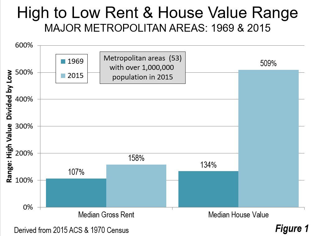
    This is illustrated by American Community Survey data for the nation’s 53 major housing markets (metropolitan areas with more than 1,000,000 residents). The range in median contract rent between the major housing markets 3.1 times, with San Jose being the most expensive and Rochester the least. The range in median house values was more than double that, at 6.6 times, between highest cost San Jose and lowest cost Pittsburgh. Thus, house prices in the most expensive markets tend to be far higher in relation to rents than in the less expensive markets.

    The rising difference between house values and rents was noted last year in The House Prices are Too Damned High, which showed that from 1969 to 2015, the difference in the range between rentals and house values rose from 51 percentage points to 375 percentage points (Figure 1). It is no coincidence that 1969 was the last census data before far more strict land use regulations were implemented in some major housing markets.
    The House Value-to-Rent Ratio

    This is illustrated by the median house value-to-rent ratio, which is calculated by dividing the median house value by the median contract rent per year (monthly times 12). Overall in 2016, the median contract rent was $841 in the United States, while the median house value was $205,000. This calculates to a value-to-rent ratio of 20.3.

    Where Housing Aspiration is Most Challenging

    California, long home to house prices far above the rest of the nation dominates the list of housing markets in which it is hardest for buyers to move up to home ownership. The worst market is the San Francisco metropolitan area, where the median house value in 2016 was nearly 40 times the median annual rent (39.6) and nearly twice the national figure of 20.3. San Jose is the second worst market, with a value-to-rent ratio of 38.7. Los Angeles is third where the median house value is 36.9 times the median annual rent. There is a larger gap down to San Diego, ranked fourth worst, where there is a median value-to-rent ratio of 31.1. Sacramento is also in the least friendly five for renters aspiring to be buyers, with a value-to-rent ratio of 29.6. This may be a surprising finding and is discussed further below. California’s other major market, Riverside-San Bernardino does better, ranking 13th worst, with a value-to-rent ratio of 24.5.

    Even with New York’s notoriously high rents, it did not muscle out California in the worst five. New York’s s value-to-rent ratio was 29.5 The balance of the 10 markets in which moving from renting to buying is most difficult also includes #7 Boston (28.1), #8 Portland (27.9), #9 Providence (27.7) and #10 Seattle (27.2).

    Comparison with Demographia Housing Affordability Ratings

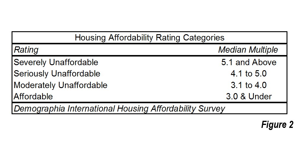
    The eleven housing markets with the highest value-to-rent ratios have ratings of “severely unaffordable” in the 13th Annual Demographia International Housing Affordability Survey. This is the least affordable rating (Figure 2) and indicates a median multiple of 5.1 or higher (median house price divided by median household income). The 12th highest value-to-rent ratio is in Salt Lake City, which is rated “seriously unaffordable,” the second most unaffordable category. Thirteenth ranked Riverside-San Bernardino was the only other severely unaffordable major U.S. housing market in the Demographia survey.

    Each of the severely unaffordable markets have land use restrictions that make it virtually impossible to build the low-cost suburban tract housing crucial to retaining housing affordability. In such markets, Buildzoon.coms’ economist Issi Romem has shown that house values have become detached from construction costs, largely the result of rising land prices (which are associated with stronger land use regulation, especially urban containment policy).
    The Surprising Case of Sacramento

    Sacramento’s high cost housing may come as a surprise. Sacramento has often “slipped under the radar” as a severely unaffordable market, yet was so from 2004 through 2008.Sacramento had reached a median multiple of 6.8 in 2005 before the housing bust and was less affordable than Vancouver, the third least affordable housing market out of nine nations rated in 2016 by Demographia. Sacramento again became severely unaffordable in last year’s Demographia survey reaching a median multiple of 5.1. But there is reason for concern in Sacramento, which has seen its median multiple rise from 2.9 to 5.1 in just four years. Any continuation of such this trend could result in a material deterioration of Sacramento’s value-to-rent ratio, made all the more likely by California’s overly restricted housing and land use regulations.

    The Value-to-Rent Ratio and Inequality

    Rising inequality is a widespread concern. Yet, as researchers have shown, much of the expanding inequality is centered in the value of owned housing, which has been associated with more restrictive land and housing regulation. In the United States, the price is being paid for by younger households, who are faced with greater student loan debts and a less lucrative economy. It is also paid for by ethnic minority households, whose more limited incomes are making the jump to home ownership even more difficult (See: Progressive Cities: Home of the Worst Housing Inequality).

    Median House Value to Median Contract Rent Ratios
    53 Major US Housing Markets (Metropolitan Areas)
    Worst Markets for Moving from Renting to Buying
    Rank Housing Market (Metropolitan Area) Value-to-Rent Ratio Median Contract Rent (Monthly) Median House Value Housing Affordabilty Rating
    1 San Francisco-Oakland, CA 39.56 $1,677 $796,100 Severely Unaffordable
    2 San Jose, CA 38.69 $1,964 $911,900 Severely Unaffordable
    3 Los Angeles, CA 36.92 $1,305 $578,200 Severely Unaffordable
    4 San Diego, CA 31.07 $1,415 $527,600 Severely Unaffordable
    5 Sacramento, CA 29.62 $1,022 $363,300 Severely Unaffordable
    6 New York, NY-NJ-PA 29.05 $1,223 $426,300 Severely Unaffordable
    7 Boston, MA-NH 28.14 $1,222 $412,700 Severely Unaffordable
    8 Portland, OR-WA 27.89 $1,031 $345,000 Severely Unaffordable
    9 Providence, RI-MA 27.77 $796 $265,300 Seriously Unaffordable
    10 Seattle, WA 27.23 $1,198 $391,500 Severely Unaffordable
    11 Denver, CO 24.79 $1,174 $349,200 Severely Unaffordable
    12 Salt Lake City, UT 24.60 $907 $267,800 Moderately Unaffordable
    13 Riverside-San Bernardino, CA 24.47 $1,086 $318,900 Severely Unaffordable
    14 Washington, DC-VA-MD-WV 23.74 $1,444 $411,400 Seriously Unaffordable
    15 Baltimore, MD 23.21 $1,055 $293,900 Moderately Unaffordable
    16 Milwaukee,WI 23.07 $737 $204,000 Seriously Unaffordable
    17 Hartford, CT 22.83 $903 $247,400 Moderately Unaffordable
    18 Raleigh, NC 22.56 $878 $237,700 Moderately Unaffordable
    19 Philadelphia, PA-NJ-DE-MD 22.27 $919 $245,600 Moderately Unaffordable
    20 Las Vegas, NV 22.06 $883 $233,700 Seriously Unaffordable
    21 Phoenix, AZ 21.97 $876 $231,000 Seriously Unaffordable
    22 Richmond, VA 21.81 $868 $227,200 Moderately Unaffordable
    23 Minneapolis-St. Paul, MN-WI 21.64 $926 $240,500 Moderately Unaffordable
    24 Virginia Beach-Norfolk, VA-NC 21.27 $940 $239,900 Moderately Unaffordable
    25 Austin, TX 21.20 $1,035 $263,300 Seriously Unaffordable
    26 Cincinnati, OH-KY-IN 21.08 $653 $165,200 Affordable
    27 Nashville, TN 21.00 $829 $208,900 Moderately Unaffordable
    28 Louisville, KY-IN 20.94 $645 $162,100 Moderately Unaffordable
    29 St. Louis,, MO-IL 20.64 $683 $169,200 Affordable
    30 Chicago, IL-IN-WI 20.60 $930 $229,900 Moderately Unaffordable
    31 Kansas City, MO-KS 20.38 $711 $173,900 Affordable
    32 Columbus, OH 20.15 $712 $172,200 Affordable
    33 Birmingham, AL 20.15 $637 $154,000 Moderately Unaffordable
    34 New Orleans. LA 19.89 $788 $188,100 Moderately Unaffordable
    35 Oklahoma City, OK 19.86 $647 $154,200 Affordable
    36 Tucson, AZ 19.82 $716 $170,300 Moderately Unaffordable
    37 Charlotte, NC-SC 19.77 $793 $188,100 Moderately Unaffordable
    38 Pittsburgh, PA 19.62 $631 $148,600 Affordable
    39 Miami, FL 19.36 $1,122 $260,600 Severely Unaffordable
    40 Grand Rapids, MI 19.20 $714 $164,500 Affordable
    41 Atlanta, GA 18.72 $880 $197,700 Moderately Unaffordable
    42 Buffalo, NY 18.63 $636 $142,200 Affordable
    43 Cleveland, OH 18.47 $659 $146,100 Affordable
    44 Indianapolis. IN 18.43 $694 $153,500 Affordable
    45 Detroit,  MI 18.37 $729 $160,700 Affordable
    46 Jacksonville, FL 18.33 $853 $187,600 Moderately Unaffordable
    47 Dallas-Fort Worth, TX 18.13 $869 $189,100 Moderately Unaffordable
    48 Orlando, FL 17.72 $948 $201,600 Seriously Unaffordable
    49 Memphis, TN-MS-AR 17.69 $671 $142,400 Moderately Unaffordable
    50 Houston, TX 17.36 $871 $181,400 Moderately Unaffordable
    51 San Antonio, TX 16.65 $802 $160,200 Moderately Unaffordable
    52 Tampa-St. Petersburg, FL 16.61 $879 $175,200 Seriously Unaffordable
    53 Rochester, NY 15.97 $725 $138,900 Affordable
    Sources: American Community Survey 2016, 13th Annual Demographia International Housing Affordability Survey.


    Wendell Cox is principal of Demographia, an international public policy and demographics firm. He is a Senior Fellow of the Center for Opportunity Urbanism (US), Senior Fellow for Housing Affordability and Municipal Policy for the Frontier Centre for Public Policy (Canada), and a member of the Board of Advisors of the Center for Demographics and Policy at Chapman University (California). He is co-author of the “Demographia International Housing Affordability Survey” and author of “Demographia World Urban Areas” and “War on the Dream: How Anti-Sprawl Policy Threatens the Quality of Life.” He was appointed to three terms on the Los Angeles County Transportation Commission, where he served with the leading city and county leadership as the only non-elected member. He served as a visiting professor at the Conservatoire National des Arts et Metiers, a national university in Paris.

    Photograph: Sacramento – One of 5 most difficult markets for moving from renting to buying.
  • Protecting Cities in Fire-Prone Regions

    If you live in a fire-prone area, which includes most of California, it is not a good idea to allow ivy and other plants to cover the sides of your building, as this winery and this church did near Santa Rosa. Both were lost to last week’s wildfires.

    Similarly, if you are a legislator in a fire-prone state, it is not a good idea to outlaw fire-resistant developments. As now-retired Forest Service researcher Jack Cohen relates in the above video, one requirement for making your home fire-safe is to have no large flammable structures within 100 feet of the home. That pretty much means people should build on one-acre or larger lots.

    But in California, the nation’s most fire-prone state, urban planners’ mania for density has led the legislature to effectively outlaw such low-density development. Santa Rosa’s Coffey Park neighborhood consisted of conventionally sized suburban homes on 50-by-100-foot lots–small for a modern suburb–resulting in many houses being only a few feet apart from one another. If one house caught fire during a dry spell, the intense radiant heat would be sure to set off the next home. As a result, the neighborhood is now a smoking ruin.

    As the Antiplanner noted a decade ago, California developers have built shelter-in-place neighborhoods that are so fire-resistant that it is safer for residents to stay in their homes than to evacuate. Wildfires have swept by these neighborhoods and not harmed a single home.

    Sadly, this technique has been criticized by even the California Department of Forestry, which argues that making homes fire-safe will just encourage people to live in fire-prone areas (meaning almost all of California). They suggested that people build their homes closer together to make them “easier to protect.” That didn’t work very well in Santa Rosa.

    If California had allowed urban areas to grow in the modern way, with density at the center and increasingly low densities at the edges, then a ring of low-density, shelter-in-place neighborhoods around Santa Rosa and other cities could have provided a fire break protecting the denser developments. But this is practically forbidden in California. So, we will get more disasters like the one in Santa Rosa and the 1991 Oakland Hills firestorm.

    This piece first appeared on The Antiplanner.

    Randal O’Toole is a senior fellow with the Cato Institute specializing in land use and transportation policy. He has written several books demonstrating the futility of government planning. Prior to working for Cato, he taught environmental economics at Yale, UC Berkeley, and Utah State University.

    Photo: Homes burned by a wildfire are seen, Oct. 11, 2017, in Santa Rosa, California via VOA News.

  • Housing Unaffordability Policies: “Paying for Dirt”

    Issi Romem, buildzoom.com’s chief economist has made a valuable contribution to the growing literature on the severe unaffordability of housing in a number of US metropolitan areas. The disparities between the severely unaffordable metropolitan areas (read San Jose, San Francisco, Los Angeles, San Diego, Portland, Seattle, Portland, Denver, Miami, New York, Boston, Sacramento and Riverside-San Bernardino) and the many more affordable areas in America are described in “Paying For Dirt: Where Have Home Values Detached From Construction Costs“. Romem points out that: “In the expensive U.S. coastal metros, home prices have detached from construction costs and can be almost four times as high as the cost of rebuilding existing structures.”

    “Paying for dirt” refers to the ballooning land costs that now comprise an unprecedented part of house values, such as in the severely unaffordable metropolitan markets above. This has created an environment where affordability is impossible. In many of these metropolitan areas, a modest house commands an exorbitant price well beyond the financial capacity of most middle income households. Land has become so expensive that it doesn’t matter what is built on it, whether the average house or a tent, the price will be too high. The market distortions are so great that Romem is able to show that, for example, the average house value in Columbus, Ohio, a delightful metropolitan area, is less than the average land value per lot in Portland (Oregon).

    The research suggests that the variation in construction costs between US metropolitan areas pales by comparison to the differences in the land costs. In the most expensive housing market, San Jose, the average house value is seven times that of Buffalo, the least expensive. By contrast, the highest cost construction market (San Francisco) is only twice as expensive as the least (Las Vegas). The land cost differences are stark, exceeding a 40 times difference in San Jose compared to Buffalo or Indianapolis. In Indianapolis, new detached house construction in 2017 was 2.5 times that of much larger and more expensive San Diego.

    The Research

    Romem’s research is similar to that of Harvard’s Edward Glaeser and Wharton’s Joseph Gyourko (“The Economic Implications of Housing Supply”), who separated US metropolitan areas into those with “well-functioning” housing markets and those without. In the well-functioning housing markets homebuilders could construct houses for what the researchers called the “minimum profitable production cost. Their list of high cost markets that are not well-functioning nearly matches Romem’s list of metropolitan areas where land costs have risen most compared to construction costs. Romem provides estimates down to the ZIP Code level in major metropolitan areas, illustrating a substantial depth of analysis.

    Consistent with Glaeser and Gyourko, Romem finds that “absent restrictions on housing supply, competition among developers tends to maintain average metropolitan home prices tethered to the cost of construction.”

    The Problem of Excessive Land Use Regulations

    In the highly regulated metropolitan areas, promoters of the urban containment policies often hide behind the fiction of topographical or geographical barriers as having created the land scarcity. A particular favorite for this blather is the San Francisco Bay Area (which includes the San Francisco and San Jose metropolitan areas) that has driven house prices up so much. There is no question that topography and geography can create such a shortage, as this photograph of Maldives capital Male shows. But nothing in the Bay Area looks like Male (photograph above).

    But San Francisco and San Jose are nothing like Male. In fact, the San Francisco Bay Area has enough land for development that millions of new houses could be constructed. San Francisco’s urbanization is dense, with at least 15 more residents per square mile than the New York urban area (population centre). Its population, nearly one-third that of New York, lives in an even smaller one-fourth the land area. There would be no need for urban containment in the Bay Area if the topography genuinely limited development.

    Toward A More Unequal Society

    In a note, Romem says that “The stark differences in land value per home are driven largely by land use policy enacted in the expensive coastal metros since the 1970s, which has inhibited these cities’ growth. These metro areas have gradually slowed down their outward expansion, i.e. they have had success in stemming sprawl, but they have failed to compensate through densification. As a result, the economic vitality of these metros has been channeled away from population growth and into housing price growth.”

    “Stemming sprawl” while maintaining housing affordability through higher densities is a time-worn theory. The record seems to indicate that it is more likely Santa will come down the chimney than density will solve the problem. There are no virtually examples of housing markets (metropolitan areas) where increasing densities has restored affordability. This is not to suggest there is no value to increased density, but rather that it is an all too convenient diversion from solutions that have a chance of working.

    Appropriately, Romem puts this childish notion to rest that increasing densities “will reduce the land value component of homes simply by dividing a fixed land value over a greater number of units.”

    The bottom line is that the house price appreciation in the high cost metropolitan areas suppresses population by “selectively determining who can and cannot afford to live there” according to Romem. This policy outcome could not be more inconsistent with encouraging economic aspiration among middle-income households, who pay the price of the greater inequality imposed by public policy. Further, those effectively “zoned out” by these policies have greater financial challenges than their parents, who generally grew up in periods of greater economic growth and were not saddled with unprecedented student loan debt.

    The financial and exclusionary challenges weigh particularly hard on the large number of disadvantaged African-Americans and Hispanics, especially those living in the most progressive cities, where pious pronouncements about affordable housing initiatives are boilerplate, but rarely amount to anything remotely substantive. In fact, distorted land and housing markets in the expensive metropolitan areas represent a colossal government failure.

    Necessary Reforms

    To the contrary, housing affordability requires well-functioning housing markets. It requires home values that have not become detached from construction costs. A minimum condition is that land use regulations not stand in the way of building low cost housing tracts on the periphery of urban areas. This does not require building on the monstrous size lots of suburban Boston, where zoning and other land use restrictions have made housing far more expensive and exclusive than it needs to be. The key is to restore the competitive market for land, so that houses on comparatively small lots, such as one-quarter or one-fifth of an acre can be built at the historic land costs (including necessary infrastructure). Glaeser and Gyourko found this factor to account for about 20 percent of final purchase prices (as did I).

    Romem expresses a hope that things will improve. “The disparity between the appearance of homes and their price tags is more than a home buyer’s gripe: it is a telltale indication of restricted housing supply. Such restrictions – rules governing land use, installed by incumbent residents or their predecessors – are exclusionary by nature and amount to the gating of access to opportunity. Hopefully, this study has helped identify where gates must be opened.”

    Indeed.

    Wendell Cox is principal of Demographia, an international public policy and demographics firm. He is a Senior Fellow of the Center for Opportunity Urbanism (US), Senior Fellow for Housing Affordability and Municipal Policy for the Frontier Centre for Public Policy (Canada), and a member of the Board of Advisors of the Center for Demographics and Policy at Chapman University (California). He is co-author of the “Demographia International Housing Affordability Survey” and author of “Demographia World Urban Areas” and “War on the Dream: How Anti-Sprawl Policy Threatens the Quality of Life.” He was appointed to three terms on the Los Angeles County Transportation Commission, where he served with the leading city and county leadership as the only non-elected member. He served as a visiting professor at the Conservatoire National des Arts et Metiers, a national university in Paris.

    Photograph: Male (capital of the Maldives): Where there are genuine topographical constraints.
    https://upload.wikimedia.org/wikipedia/commons/6/67/Male_maldives.jpg

  • San Francisco’s Abundant Developable Land Supply

    The San Francisco Bay Area (home of the San Francisco and San Jose metropolitan areas), which has often been cited as a place where natural barriers have left little land for development. This is an impression easily obtained observing the fairly narrow strips of urbanization on both sides of San Francisco Bay, hemmed in by hills.

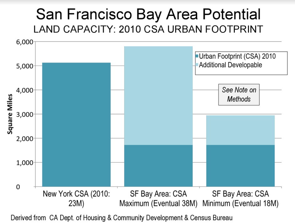
    However the Bay Area’s urbanization long ago leapt over the most important water bodies and then the Berkeley Hills to the east. Not only is the San Francisco Bay Area CSA high density, but it is also spatially small. In 2016, the San Francisco built-up urban area was only the 23rd largest in land area in the world. New York, the world’s largest built-up urban area in geographical expanse is more than four times as large.

    There is plenty of developable land in the San Francisco Bay Area. Data in a 1997 state analysis indicated that another 1,500 to 4,300 square miles (3,900 to 11,000 square kilometers) could be developed in the Bay Area CSA. The lower bound assumed no farmland conversion and stringent environmental regulation. The report also found that in recent years, residential development had become marginally denser, yet not incompatible with the detached housing remains the preference in California (Figure). The state has more than enough developable land for future housing needs.

    Demographia International Housing Affordability Survey with a median multiple of 9.6 (median house price divided by median household income) and the San Francisco metropolitan area is 7th worst, with a median multiple of 9.2. Before the evolution toward urban containment policies began, the median multiples in these metropolitan areas (and virtually all in the United States) were around 3.0 or less.
    The decades old Bay Area housing affordability crisis, and that of other urban containment metropolitan areas that are now seriously unaffordable (median multiples over 5.0) seeking to force higher densities, is more the result of policy than nature.

    Note on Method: Some of the CSA urban population is not in the continuous urbanization of San Francisco-San Jose built-up urban area, such as in the Santa Rosa, Stockton and Santa Cruz urban areas. This analysis is based on data from the California Department of Housing and Community Development and the U.S. Census Bureau. It is based on an estimate of additional development occurring from 1996 to 2010 and the land remaining after deduction of recently developed land. The population capacity assumes the “marginally higher” densities used by the California Department of Housing and Community Development, which it notes would not require substantial changes in the “current form of housing development” (1997).

  • Rising Rents Are Stressing Out Tenants And Heightening America’s Housing Crisis

    The home-buying struggles of Americans, particularly millennials, have been well documented. Yet a recent study by Hunt.com found that the often-proposed “solution” of renting is not much of a panacea. Rents as a percentage of income, according to Zillow, are now at a historic high of 29.1%, compared with the 25.8% rate that prevailed from 1985 to 2000.

    No surprise, then, that 58% of the 1,300 renters in the Hunt survey said they felt “stressed” about their rent, or that many respondents said they couldn’t save for future purchases like homes. Rather than the sunny freedom promised by those who promote a “rentership society,” most of those surveyed said that finding a convenient place with the amenities they required – for example, fitness rooms, places for pets and adequate space – was very difficult. Some renters have been forced to euthanize their pets, spend upwards of 50 days looking for a place or move farther from family and friends.

    All of this is taking place at a time when the national vacancy rate has fallen to 7.3% (in the second quarter of 2017), from 11.1% in the third quarter of 2009. That trend has continued even with apartment construction in many areas, notably core cities, because the new buildings tend to be too expensive for most renters.

    Fuel for a Housing Crisis

    There is a strong relationship between high rents and high house prices. Although rents have not risen as much as house prices generally, they tend to attract people who in the past might have become homeowners but instead have been crowded out by the high prices. This essentially brings into the rental market more affluent tenants who directly compete with those with lower incomes.

    The result in many places, such as Southern California, is overcrowding. Two-thirds of the places in the United States (municipalities and census-designated places) with more than 5,000 residences and with more than 10% of housing units being overcrowded are in California, according to the American Community Survey.

    The rent-related stress also points to a bigger crisis: the decline in the purchase of homes. One of the most prominent reasons for not buying a house directly relates to higher rents: It becomes all but impossible to save enough for a down payment. This also reflects changes in the labor market; service and blue-collar workers, whose incomes have been down in relation to rents, are the most burdened by rising rents. In San Francisco, even a teacher has been driven into the ranks of the homeless.

    The situation is worst in the most expensive markets. In New York City, incomes for millennials (ages 18–29) have dropped in real terms compared with the same age cohort in 2000, despite considerably higher education levels, while rents have increased 75%. New York, Los Angeles and San Francisco have three of the nation’s four lowest homeownership rates for young people and among the lowest birthrates.

    According to Zillow, for workers ages 22-34, rent costs claim up to 45% of income in the Los Angeles, San Francisco, New York and Miami metropolitan areas, compared with closer to 30% of income in metros like Dallas-Fort Worth and Houston. Home prices provide an even starker contrast. Dallas-Fort Worth, the nation’s fastest-growing housing market, as well as Houston, San Antonio and Charlotte have prices that are more like one-third those of the superstars.

    That helps explain why, according to the Hunt survey, the highest percentage of people who cannot save for future purchases (almost 60%) live on the pricey West Coast. The West Coast also had the largest percentage of people stressed about their rent, followed, not surprisingly, by the East Coast.

    High rents may also help explain recent shifts in migration to lower-rent areas. A recent survey by Apartmentalist.com found that the best prospects for renters becoming homeowners are in metropolitan areas like Pittsburgh, Provo, Madison, San Antonio, Columbus, Oklahoma City and Houston; the worst are, not surprisingly, in California, New York, Boston and Miami.

    Profound Implications

    What emerges from the Hunt study, and other research, is a renting population that may never achieve homeownership. This represents a sort of social evolution from the culture of self-assertion and independence that once so clearly characterized America after World War II and was so important to the unprecedented spread of middle-income affluence. Rather than striking out on their own, many millennials are simply failing to launch, with record numbers living with their parents or forced to shell out much of their income rent.

    The implications of high rent, and declining home ownership, could be profound over time. In survey after survey, a clear majority of millennials — roughly 80%, including the vast majority of renters — express interest in acquiring a home of their own. A Fannie Mae survey of people under 40 found that nearly 80% of renters thought that owning made more financial sense, a sentiment shared by an even larger number of owners. They cited such things as asset appreciation, control over the living environment and a hedge against rent increases.

    But it won’t just be renters impacted by rising rents. Jason Furman, who served as chairman of the Council of Economic Advisors under President Obama, calculated that a single-family home contributed two and a half times as much to the national GDP as an apartment unit.

    The decline in investment in residential properties has dropped to levels not seen since World War II. By some estimates, if we had that kind of housing investment again, we would return to 4% growth, as opposed to our all-too-familiar 2% and below.

    America’s housing crisis, long tied to ownership, is now extending into rising rents. But the stress that renters are feeling impacts all of us.

    This piece originally appeared on Forbes.com.

    Joel Kotkin is executive editor of NewGeography.com. He is the Roger Hobbs Distinguished Fellow in Urban Studies at Chapman University and executive director of the Houston-based Center for Opportunity Urbanism. His newest book is The Human City: Urbanism for the rest of us. He is also author of The New Class ConflictThe City: A Global History, and The Next Hundred Million: America in 2050. He lives in Orange County, CA.

    Wendell Cox is principal of Demographia, an international public policy and demographics firm. He is a Senior Fellow of the Center for Opportunity Urbanism (US), Senior Fellow for Housing Affordability and Municipal Policy for the Frontier Centre for Public Policy (Canada), and a member of the Board of Advisors of the Center for Demographics and Policy at Chapman University (California). He is co-author of the “Demographia International Housing Affordability Survey” and author of “Demographia World Urban Areas” and “War on the Dream: How Anti-Sprawl Policy Threatens the Quality of Life.” He was appointed to three terms on the Los Angeles County Transportation Commission, where he served with the leading city and county leadership as the only non-elected member. He served as a visiting professor at the Conservatoire National des Arts et Metiers, a national university in Paris.

    Photo: Omar Bárcena, via Flickr, using CC License.

  • How We Are Kluging the World’s Growth Process

    The quirks of software and operating systems that we seem to experience on a daily basis are the result of Kluges – almost all software is written with fixes that work for a particular problem, often without knowing exactly why that fix works. As both a land planner and developer of high level precision design and engineering software, I do not allow kluged fixes – for either business.

    Why do kluges exist?

    Kluges are rampant in software and hardware development.


    A kluge is a quick and easy fix to one problem, but hardware and software design is very complex, so what might fix one problem can have dramatic negative effects elsewhere. The potential of a larger problem occurring with a kluged fix is very real, and everyone suffers because what ‘seems to work’ on a particular problem may have a domino effect for things that could not be foreseen in normal testing.

    What other industry has rampant kluges?

    Subdividing land!

    Kluge #1: A new subdivision is more than likely designed by the local civil engineer who is unlikely to possess a strong neighborhood design background. This is because the firm who plans the development will also get the lucrative engineering and surveying work. For that reason, every engineering firm, and most land surveying firms boast of their land planning abilities, even if there are no qualified and experienced ‘neighborhood’ designers on staff.

    Kluge #2: Assuming the local consultants relationship with the staff, council, and planning commission will result in a better development for the developer and builder – and a better city. The local consultant will likely have a familiarity with the people involved in the approval process, but may be far too easy compliant with every demand and change – no matter how absurd, than to argue a valid point with the city. They may know the design or idea is superior to the same old way things are done, but will try to convince the developer (who is paying for their services) the good idea is a bad idea. Progress stagnates – and this a major reason many new subdivisions looks the same (or worse) than one designed in the 1960’s.

    Kluge #3: The cities’ regulations. Cities have in-house staff or hire outside consultants to maintain and update their regulations which are essentially a boiler-plate document of the adjacent city. Nothing in the regulations reward developers for doing a better job. Will the development be an asset or an instant slum? If it meets the minimums – it must be approved! That’s it.

    Smart Code? There is nothing smart about this dumb idea – it only guarantees the consultant pushing these incredibly complex and restrictive codes is forever retained to consult at every city meeting. Overly restrictive code guarantees mindless replication and places a roadblock to progress and innovation.

    Kluge# 4: Technology used to develop land. I’ve been developing and marketing civil engineering, surveying, and design software for almost four decades. On a sales call – what do you think is the first question? How much faster can we get our work out? What’s the question I’ve never heard? How much better can we design our neighborhoods for our clients and those that will live within? The billions of dollars spent on CAD and GIS technology, training, updates, hardware, and support has resulted in zero difference in the actual pattern of growth! City planning commissions and councils are presented the same 2D plans that nobody can understand and visualize. Virtually unchanged since 1960, but presented in PowerPoint instead of transparency slides on an overhead projector.

    Kluge #5: The land development consulting industry itself. I know of no other industry where the main design professionals (architects, planners, engineers, surveyors, etc.) are less likely to collaborate and communicate to assure the end user (the resident or business owner) is best served. There are many reasons why this is such a dysfunctional industry. The professionals involved have completely different skillsets. They often conflict with the others’ skillsets. All this can be solved with a new era of consulting industry where all involved have a common knowledge base to begin with – somewhat like the medical industry. This leads us to the next kluge…

    Kluge #6: The universities only teach a narrow focus on an isolated aspect of the development process. With a ‘common knowledge base’ where a student will learn all aspects with technology and systems that can advance the industry we can tear down the barriers of communication and build collaboration. One major problem: the professors. They will need to harness better technologies and re-learn themselves – making an effort and need to communicate and collaborate among themselves.

    Kluge #7: What happened to teaching – design? The world has morphed down to only a few major players in the software industry who have done nothing to advance the growth and redevelopment process through research and innovation. Over generations, gradually the world loses skillsets that were commonplace before computers existed. This is why all those new apartment projects and commercial buildings look the same, and that new subdivision is more mundane and cookie-cutter than in the past.

    Kluge #8: Traffic regulations and trendy roundabouts. Don’t even try to convince me that roundabouts are a good idea, they are not. Of the well over 1,000 neighborhoods I’ve designed this past 26 years I’ve included a total of 3 roundabouts. There are much better alternatives that are safer and maintain flow, reducing time and energy while increasing safety.

    Have you ever passed a restaurant thinking you are a bit hungry, but then decide to pass it up because you are routed a ridiculously long distance of multiple intersections to the place and instead pass it by? We all have. Instead of making access more efficient and convenient, often these rules do quite the opposite. As a pedestrian or on your bike have you ever tried to cross at a roundabout? Did you feel safer than at a signalized intersection? Progress? No. Kluge? Yes. Thus roundabouts are safer for pedestrians because most go far out of their way to avoid crossing them!

    Kluge #9: Streets as the pedestrian route. Subdividing land is all about density – little about function. The pattern assures the most units (housing or commercial square footage) are sardined into a site. This pattern sets the street first – lots second. Nothing else. Pretty simple and quick with the latest technology (kluge #4). What of the streetscape (curb appeal, monotony)? What’s the views from within the home to adjacent open space? What open space? How easy is it to walk through the neighborhood to destinations you would want to walk or ride a bike to? Walks that simply follow the internal streets are highly unlikely to make a stroll convenient, thus the mindless walks designed automatically in CAD will discourage a stroll. To fix this deficiency, the vehicular and the pedestrian routes should be two different systems, merging where it makes sense.

    Kluge #10: Revisions along the approval process. Suppose, an experienced and talented land planner carefully thought through the design of the neighborhood. The traffic entering maintains flow along streets void of monotony. There is a separate and connective pedestrian system, and the site plan follows the natural terrain honoring natures design, while reducing run-off and earthwork – which in turn saves the trees. At the first public meeting, the neighbors complain about traffic and the city planner demands you not connect at the proposed locations and add some new connections. You make small changes and as a result your traffic no longer flows as the planner designed. The engineer simply complies (see kluge #2). The length of the cul-de-sac is 70 feet longer than allowed, and will need to be adjusted, but that destroys the placement on top of a knoll which makes more sense, and the main trail connecting through the cul-de-sac is rerouted which destroys the pedestrian connectivity.

    As a software developer and president of my company I do not allow kluges. The LandMentor system we developed has taken 12 years, mostly because it’s kluge free. I seriously doubt there is any software of any type that exists that has a 12 year initial development process. What we learned from the software business applies to land development and home design (single family and multifamily) – when problems arise or revisions are demanded, it’s most often better to start afresh than force an older ‘invested’ idea to work, the very definition of a kluge.

    There is no quick fix to sustainable development, and no place for kluges.

    Rick Harrison is President of Rick Harrison Site Design Studio and Neighborhood Innovations, LLC. He is author of Prefurbia: Reinventing The Suburbs From Disdainable To Sustainable and creator of LandMentor. His websites are rhsdplanning.com and LandMentor.com

    Photo: Zoedovemany (Own work) [CC BY-SA 4.0], via Wikimedia Commons

  • Progressive Cities: Home of the Worst Housing Inequality

    America’s most highly regulated housing markets are also reliably the most progressive in their political attitudes. Yet in terms of gaining an opportunity to own a house, the price impacts of the tough regulation mean profound inequality for the most disadvantaged large ethnicities, African-Americans and Hispanics.

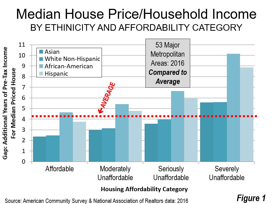
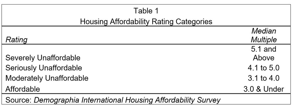
    Based on the housing affordability categories used in the Demographia International Housing Affordability Survey for 2016 (Table 1), housing inequality by ethnicity is the worst among the metropolitan areas rated “severely unaffordable.” In these 11 major metropolitan area markets, the most highly regulated, median multiples (median house price divided by median household income) exceed 5.0. For African-Americans, the median priced house is 10.2 times median incomes. This is 3.7 more years of additional income than the overall average in these severely unaffordable markets, where median house prices are 6.5 times median household incomes. It is only marginally better for Hispanics, with the median price house at 8.9 times median household incomes, 2.4 years more than the average in these markets (Figure 1).

    The comparisons with the 13 affordable markets (median multiples of 3.0 and less) is even more stark. For African-American households things are much better than in the more progressive and most expensive metropolitan areas. The median house prices is equal to 4.6 years of median income, 5.5 years less than in the severely affordable markets. Moreover, for African-Americans, housing affordability is only marginally worse than the national average in the affordable market.

    Things are even better for Hispanics, who would find the median house price 3.8 times median incomes, 5.1 years less than in the severely affordable markets. This is better than the national average housing affordability.

    Among the four markets rated “seriously unaffordable,” (median multiple from 4.1 to 5.0) the inequality is slightly less, with African-Americans finding median house prices equal to 2.2 years of additional income compared to average. The disadvantage for Hispanics is 1.5 years.

    In contrast, inequality is significantly reduced in the less costly “moderately unaffordable” markets (median multiple of 3.1 to 4.0) and the “affordable” markets (median multiple of 3.0 and less).

    The discussion below describes the 10 largest and smallest housing affordability gaps for African-American and Hispanic households relative to the average household, within the particular metropolitan markets. The gaps within ethnicities compared to the affordable markets would be even more. The four charts all have the same scale (a top housing affordability gap of 10 years) for easy comparison.

    able 2 illustrates housing affordability gaps by major metropolitan areas. There are also housing affordability ranking gap tables by African-American households (Table 3) and Hispanic households (Table 4).

    Largest Housing Affordability Gaps: African American

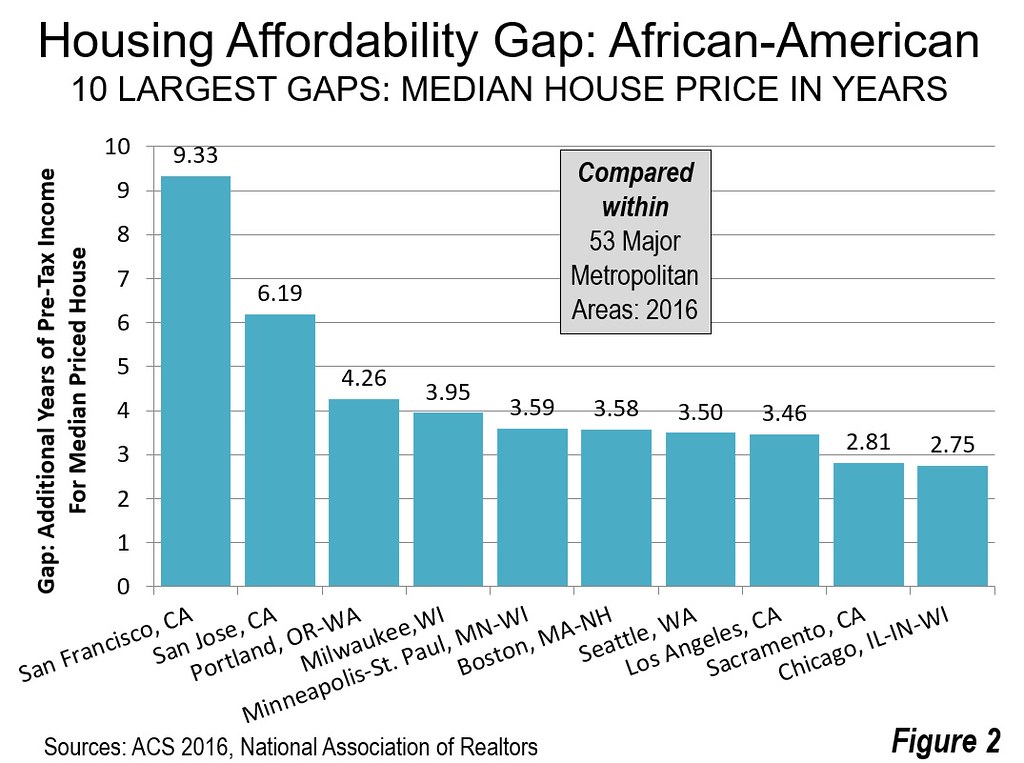
    African-Americans have the largest housing affordability inequality gap. And these gaps are most evident in some of the nation’s most progressive cities. The largest gap is in San Francisco, where the median income African-American household faces median house prices that are 9.3 years of income more than the average. In nearby San Jose ranks the second worst, where the gap is 6.2 years. Overall, the San Francisco Bay Area suffers by far the area of least housing affordability for African-Americans compared to the average household.

    Portland, long the darling of the international urban planning community, ranks third worst, where the median income African-American household to purchase the median priced house. Milwaukee and Minneapolis – St. Paul ranked fourth and fifth worst followed by Boston, Seattle, Los Angeles, Sacramento and Chicago (Figure 2).

    Largest Housing Affordability Gaps: Hispanics

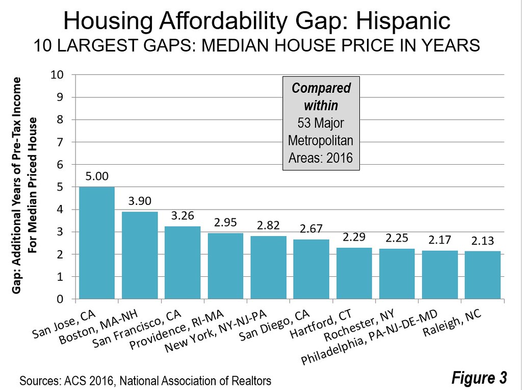
    Two of the three worst positions are occupied by the two metropolitan areas in the San Francisco Bay Area. The worst housing affordability gap for Hispanics is in San Jose, a more than one-quarter Hispanic metropolitan area where the median income Hispanic household would require 5.0 years of additional income to pay for the median priced house compared to the average. Boston ranks second worst at 3.9. San Francisco third worst at 3.3 years. Providence and New York rank fourth and fifth worst. The second five worst housing inequality for Hispanics is in San Diego, Hartford, Rochester, Philadelphia and Raleigh (Figure 3).

    The San Francisco Bay Area: “Inequality City”

    Perhaps no part of the country is more renowned for its progressive politics and politicians than the San Francisco Bay Area. Yet, in housing equality, the Bay Area is anything but progressive. If the African-American and Hispanic housing inequality measures are averaged, disadvantaged minorities face house prices that average approximately 6.25 years more years of median income in San Francisco and 5.60 more years of median income in San Jose.

    Moreover, no one should imagine that recent state law authorizing a $4 billion “affordable housing” bond election will have any significant impact. According to the Sacramento Bee, voter approval would lead to 70,000 new housing units annually, when the need for low and very low income households is 1.5 million. The bond issue would do virtually nothing for the many middle-income households who are struggling to pay the insanely high housing costs California’s regulatory nightmare has developed.

    Smallest Housing Affordability Gaps: African-American

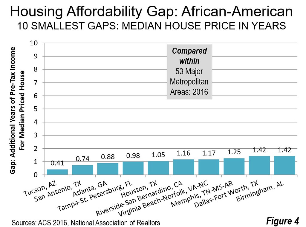
    Tucson has the smallest housing affordability gap for African-Americans. In Tucson, the median income African-American household would pay approximately 0.4 years (four months) more in income for the median priced house than the average household. In San Antonio, Atlanta and Tampa – St. Petersburg, the housing affordability gaps are under 1.0. Houston, Riverside – San Bernardino, Virginia Beach – Norfolk, Memphis, Dallas – Fort Worth and Birmingham round out the second five. It may be surprising that eight of the metropolitan areas with the smallest housing affordability gaps for African-Americans are in the South and perhaps most surprisingly of all that one of the best, at number 10, is Birmingham. (Figure 4).

    Smallest Housing Affordability Gaps: Hispanic

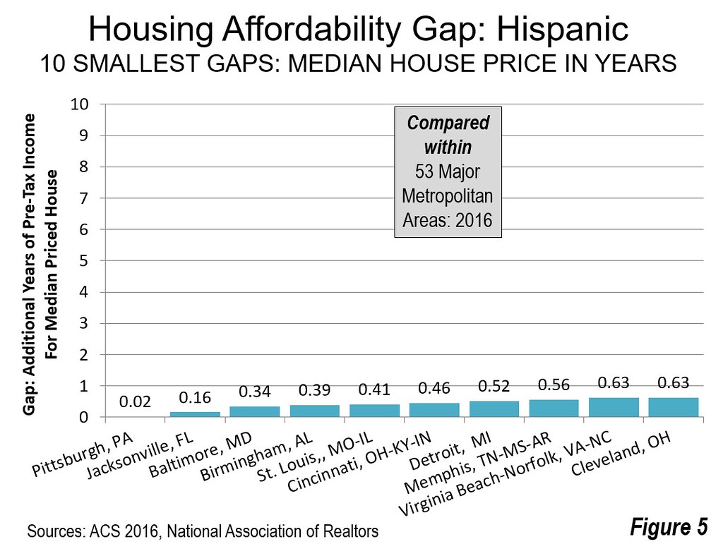
    Among Hispanic households, the smallest housing affordability gap is in Pittsburgh, where the median priced house would require less than 10 days more in median income for a Hispanic household compared the overall average. In Jacksonville the housing affordability gap for Hispanics would be less than two months. In Baltimore, Birmingham, St. Louis and Cincinnati, the median house price is the equivalent of less than six months of median income for an Hispanic household. Detroit, Memphis, Virginia Beach – Norfolk and Cleveland round out the ten smallest housing affordability gaps for Hispanics (Figure 5).

    Housing Affordability is the Best for Asians

    Recent American Community Survey data indicated that Asians have median household incomes a quarter above those of White Non-– Hispanics. This advantage is also illustrated in the housing affordability data. Asians have better housing affordability than White Non-– Hispanics in 37 of the 53 major metropolitan areas (over 1 million population).

    The Importance of Housing Opportunity

    Housing opportunity is important. African-Americans and Hispanics already face challenges given their generally lower incomes. However, by no serious political philosophy, progressive or otherwise, should any ethnicity find themselves even further disadvantaged by political barriers, such as have been created by over-zealous land and housing regulators.

    Wendell Cox is principal of Demographia, an international public policy and demographics firm. He is a Senior Fellow of the Center for Opportunity Urbanism (US), Senior Fellow for Housing Affordability and Municipal Policy for the Frontier Centre for Public Policy (Canada), and a member of the Board of Advisors of the Center for Demographics and Policy at Chapman University (California). He is co-author of the “Demographia International Housing Affordability Survey” and author of “Demographia World Urban Areas” and “War on the Dream: How Anti-Sprawl Policy Threatens the Quality of Life.” He was appointed to three terms on the Los Angeles County Transportation Commission, where he served with the leading city and county leadership as the only non-elected member. He served as a visiting professor at the Conservatoire National des Arts et Metiers, a national university in Paris.

    Table 2
    Housing Affordability Gap by Ethnicity: 2016
    53 Major Metropolitan Areas (Over 1,000,000 Population)
    Median Multiple (Median house price divided by median household income)
    MSA Median Multiple: All Households Median Multiple: African-American African American Housing Affordability Gap in Years Ranked Most to Least Equal: African-American Median Multiple:
    Hispanic
    Hispanic Housing Affordability Gap in Years Ranked Most to Least Equal: Hispanic Exhibit: Median Multiple: Asian Exhibit: Median Multiple: White Non-Hispanic
       
     Atlanta, GA       2.95          3.83           0.88              3        3.65          0.70           13       2.30            2.45
     Austin, TX       4.00          5.69           1.69            19        5.04          1.04           24       3.23            3.52
     Baltimore, MD       3.29          4.75           1.46            12        3.64          0.34             3       2.60            2.83
     Birmingham, AL       3.57          4.99           1.42            10        3.96          0.39             4       2.95            3.02
     Boston, MA-NH       5.11          8.69           3.58            47        9.02          3.90           52       4.67            4.62
     Buffalo, NY       2.48          4.79           2.32            38        4.58          2.10           43       2.90            2.20
     Charlotte, NC-SC       3.47          4.95           1.47            13        4.77          1.30           32       2.31            3.08
     Chicago, IL-IN-WI       3.56          6.30           2.75            43        4.45          0.90           20       2.69            2.94
     Cincinnati, OH-KY-IN       2.53          4.70           2.17            35        2.99          0.46             6       1.75            2.33
     Cleveland, OH       2.54          4.50           1.96            27        3.17          0.63           10       1.49            2.16
     Columbus, OH       2.91          4.78           1.87            24        4.10          1.19           30       2.50            2.68
     Dallas-Fort Worth, TX       3.56          4.98           1.42              9        4.70          1.14           26       2.55            2.87
     Denver, CO       5.34          7.64           2.29            37        7.40          2.05           42       5.33            4.76
     Detroit,  MI       4.01          6.71           2.70            41        4.53          0.52             7       2.56            3.48
     Grand Rapids, MI       2.68          4.66           1.98            28        3.85          1.16           28       2.95            2.53
     Hartford, CT       3.18          4.88           1.70            20        5.48          2.29           47       2.78            2.82
     Houston, TX       3.52          4.57           1.05              5        4.68          1.15           27       2.54            2.65
     Indianapolis. IN       2.82          4.89           2.07            31        4.45          1.63           38       2.48            2.50
     Jacksonville, FL       3.71          5.15           1.43            11        3.88          0.16             2       3.32            3.38
     Kansas City, MO-KS       2.95          4.96           2.00            30        3.97          1.02           23       2.64            2.68
     Las Vegas, NV       4.37          6.36           1.98            29        5.19          0.82           16       3.63            3.85
     Los Angeles, CA       7.69        11.15           3.46            45        9.74          2.05           41       6.68            6.03
     Louisville, KY-IN       2.99          4.90           1.91            25        3.92          0.93           21       2.48            2.71
     Memphis, TN-MS-AR       3.12          4.37           1.25              8        3.68          0.56             8       2.13            2.29
     Miami, FL       5.94          7.58           1.64            17        6.64          0.70           12       4.39            4.68
     Milwaukee,WI       3.93          7.88           3.95            49        5.79          1.86           40       2.78            3.33
     Minneapolis-St. Paul, MN-WI       3.24          6.83           3.59            48        4.64          1.40           34       3.25            3.01
     Nashville, TN       3.74          5.43           1.69            18        5.04          1.30           33       3.12            3.43
     New Orleans. LA       3.85          6.42           2.57            40        5.02          1.17           29       4.01            2.93
     New York, NY-NJ-PA       5.40          7.85           2.45            39        8.22          2.82           49       4.68            4.25
     Oklahoma City, OK       2.74          4.81           2.07            32        3.62          0.88           19       2.52            2.45
     Orlando, FL       4.28          6.00           1.72            22        5.21          0.94           22       2.93            3.60
     Philadelphia, PA-NJ-DE-MD       3.42          5.69           2.28            36        5.59          2.17           45       3.02            2.82
     Phoenix, AZ       4.01          5.54           1.53            14        5.07          1.06           25       3.17            3.62
     Pittsburgh, PA       2.68          4.61           1.93            26        2.70          0.02             1       1.97            2.54
     Portland, OR-WA       5.11          9.38           4.26            50        6.69          1.57           37       4.44            4.89
     Providence, RI-MA       4.26          6.38           2.12            34        7.21          2.95           50       3.09            3.95
     Raleigh, NC       3.46          5.01           1.56            15        5.59          2.13           44       2.47            3.12
     Richmond, VA       3.74          5.44           1.70            21        4.61          0.87           18       2.75            3.14
     Riverside-San Bernardino, CA       5.38          6.55           1.16              6        6.04          0.66           11       4.04            4.85
     Rochester, NY       2.42          4.52           2.10            33        4.67          2.25           46       2.26            2.21
     Sacramento, CA       5.00          7.81           2.81            44        6.21          1.21           31       4.63            4.46
     St. Louis,, MO-IL       2.74          4.46           1.72            23        3.15          0.41             5       2.41            2.45
     Salt Lake City, UT       4.00  No data           5.49          1.49           36       3.70            3.77
     San Antonio, TX       3.69          4.43           0.74              2        4.41          0.72           15       2.89            2.86
     San Diego, CA       7.98        10.72           2.74            42      10.65          2.67           48       6.88            6.94
     San Francisco-Oakland, CA       8.67        18.01           9.33            52      11.93          3.26           51       7.96            7.29
     San Jose, CA       9.09        15.28           6.19            51      14.08          5.00           53       7.80            8.24
     Seattle, WA       5.27          8.77           3.50            46        7.02          1.74           39       4.55            5.00
     Tampa-St. Petersburg, FL       3.87          4.86           0.98              4        4.74          0.87           17       2.85            3.65
     Tucson, AZ       4.00          4.41           0.41              1        4.71          0.71           14       4.17            3.54
     Virginia Beach-Norfolk, VA-NC       3.48          4.65           1.17              7        4.11          0.63             9       2.94            3.00
     Washington, DC-VA-MD-WV       4.08          5.64           1.57            16        5.54          1.46           35       3.76            3.38
     Overall median multiple from Demographia International Housing Affordability Survey: Updated with revised income data from 2016 ACS. 
     Median multiple: Median house price divided by median household income 
    Table 3
    African-American Housing Affordability Gap Ranked: Most to Least Equal 
    53 Major Metropolitan Areas (Over 1,000,000 Population)
    Median Multiple (Median house price divided by median household income)
    MSA Median Multiple: All Households Median Multiple: African-American African American Housing Affordability Gap in Years Ranked Most to Least Equal: African-American Median Multiple:
    Hispanic
    Hispanic Housing Affordability Gap in Years Ranked Most to Least Equal: Hispanic Exhibit: Median Multiple: Asian Exhibit: Median Multiple: White Non-Hispanic
     
     Tucson, AZ       4.00          4.41           0.41              1        4.71          0.71           14       4.17            3.54
     San Antonio, TX       3.69          4.43           0.74              2        4.41          0.72           15       2.89            2.86
     Atlanta, GA       2.95          3.83           0.88              3        3.65          0.70           13       2.30            2.45
     Tampa-St. Petersburg, FL       3.87          4.86           0.98              4        4.74          0.87           17       2.85            3.65
     Houston, TX       3.52          4.57           1.05              5        4.68          1.15           27       2.54            2.65
     Riverside-San Bernardino, CA       5.38          6.55           1.16              6        6.04          0.66           11       4.04            4.85
     Virginia Beach-Norfolk, VA-NC       3.48          4.65           1.17              7        4.11          0.63             9       2.94            3.00
     Memphis, TN-MS-AR       3.12          4.37           1.25              8        3.68          0.56             8       2.13            2.29
     Dallas-Fort Worth, TX       3.56          4.98           1.42              9        4.70          1.14           26       2.55            2.87
     Birmingham, AL       3.57          4.99           1.42            10        3.96          0.39             4       2.95            3.02
     Jacksonville, FL       3.71          5.15           1.43            11        3.88          0.16             2       3.32            3.38
     Baltimore, MD       3.29          4.75           1.46            12        3.64          0.34             3       2.60            2.83
     Charlotte, NC-SC       3.47          4.95           1.47            13        4.77          1.30           32       2.31            3.08
     Phoenix, AZ       4.01          5.54           1.53            14        5.07          1.06           25       3.17            3.62
     Raleigh, NC       3.46          5.01           1.56            15        5.59          2.13           44       2.47            3.12
     Washington, DC-VA-MD-WV       4.08          5.64           1.57            16        5.54          1.46           35       3.76            3.38
     Miami, FL       5.94          7.58           1.64            17        6.64          0.70           12       4.39            4.68
     Nashville, TN       3.74          5.43           1.69            18        5.04          1.30           33       3.12            3.43
     Austin, TX       4.00          5.69           1.69            19        5.04          1.04           24       3.23            3.52
     Hartford, CT       3.18          4.88           1.70            20        5.48          2.29           47       2.78            2.82
     Richmond, VA       3.74          5.44           1.70            21        4.61          0.87           18       2.75            3.14
     Orlando, FL       4.28          6.00           1.72            22        5.21          0.94           22       2.93            3.60
     St. Louis,, MO-IL       2.74          4.46           1.72            23        3.15          0.41             5       2.41            2.45
     Columbus, OH       2.91          4.78           1.87            24        4.10          1.19           30       2.50            2.68
     Louisville, KY-IN       2.99          4.90           1.91            25        3.92          0.93           21       2.48            2.71
     Pittsburgh, PA       2.68          4.61           1.93            26        2.70          0.02             1       1.97            2.54
     Cleveland, OH       2.54          4.50           1.96            27        3.17          0.63           10       1.49            2.16
     Grand Rapids, MI       2.68          4.66           1.98            28        3.85          1.16           28       2.95            2.53
     Las Vegas, NV       4.37          6.36           1.98            29        5.19          0.82           16       3.63            3.85
     Kansas City, MO-KS       2.95          4.96           2.00            30        3.97          1.02           23       2.64            2.68
     Indianapolis. IN       2.82          4.89           2.07            31        4.45          1.63           38       2.48            2.50
     Oklahoma City, OK       2.74          4.81           2.07            32        3.62          0.88           19       2.52            2.45
     Rochester, NY       2.42          4.52           2.10            33        4.67          2.25           46       2.26            2.21
     Providence, RI-MA       4.26          6.38           2.12            34        7.21          2.95           50       3.09            3.95
     Cincinnati, OH-KY-IN       2.53          4.70           2.17            35        2.99          0.46             6       1.75            2.33
     Philadelphia, PA-NJ-DE-MD       3.42          5.69           2.28            36        5.59          2.17           45       3.02            2.82
     Denver, CO       5.34          7.64           2.29            37        7.40          2.05           42       5.33            4.76
     Buffalo, NY       2.48          4.79           2.32            38        4.58          2.10           43       2.90            2.20
     New York, NY-NJ-PA       5.40          7.85           2.45            39        8.22          2.82           49       4.68            4.25
     New Orleans. LA       3.85          6.42           2.57            40        5.02          1.17           29       4.01            2.93
     Detroit,  MI       4.01          6.71           2.70            41        4.53          0.52             7       2.56            3.48
     San Diego, CA       7.98        10.72           2.74            42      10.65          2.67           48       6.88            6.94
     Chicago, IL-IN-WI       3.56          6.30           2.75            43        4.45          0.90           20       2.69            2.94
     Sacramento, CA       5.00          7.81           2.81            44        6.21          1.21           31       4.63            4.46
     Los Angeles, CA       7.69        11.15           3.46            45        9.74          2.05           41       6.68            6.03
     Seattle, WA       5.27          8.77           3.50            46        7.02          1.74           39       4.55            5.00
     Boston, MA-NH       5.11          8.69           3.58            47        9.02          3.90           52       4.67            4.62
     Minneapolis-St. Paul, MN-WI       3.24          6.83           3.59            48        4.64          1.40           34       3.25            3.01
     Milwaukee,WI       3.93          7.88           3.95            49        5.79          1.86           40       2.78            3.33
     Portland, OR-WA       5.11          9.38           4.26            50        6.69          1.57           37       4.44            4.89
     San Jose, CA       9.09        15.28           6.19            51      14.08          5.00           53       7.80            8.24
     San Francisco-Oakland, CA       8.67        18.01           9.33            52      11.93          3.26           51       7.96            7.29
     Salt Lake City, UT       4.00  No data         5.49          1.49           36       3.70            3.77
     Overall median multiple from Demographia International Housing Affordability Survey: Updated with revised income data from 2016 ACS. 
     Median multiple: Median house price divided by median household income 
    Table 4
    Hispanic Housing Affordability Gap Ranked: Most to Least Equal 
    53 Major Metropolitan Areas (Over 1,000,000 Population)
    Median Multiple (Median house price divided by median household income)
    MSA Median Multiple: All Households Median Multiple: African-American African American Housing Affordability Gap in Years Ranked Most to Least Equal: African-American Median Multiple:
    Hispanic
    Hispanic Housing Affordability Gap in Years Ranked Most to Least Equal: Hispanic Exhibit: Median Multiple: Asian Exhibit: Median Multiple: White Non-Hispanic
       
     Pittsburgh, PA       2.68          4.61           1.93            26        2.70          0.02             1       1.97            2.54
     Jacksonville, FL       3.71          5.15           1.43            11        3.88          0.16             2       3.32            3.38
     Baltimore, MD       3.29          4.75           1.46            12        3.64          0.34             3       2.60            2.83
     Birmingham, AL       3.57          4.99           1.42            10        3.96          0.39             4       2.95            3.02
     St. Louis,, MO-IL       2.74          4.46           1.72            23        3.15          0.41             5       2.41            2.45
     Cincinnati, OH-KY-IN       2.53          4.70           2.17            35        2.99          0.46             6       1.75            2.33
     Detroit,  MI       4.01          6.71           2.70            41        4.53          0.52             7       2.56            3.48
     Memphis, TN-MS-AR       3.12          4.37           1.25              8        3.68          0.56             8       2.13            2.29
     Virginia Beach-Norfolk, VA-NC       3.48          4.65           1.17              7        4.11          0.63             9       2.94            3.00
     Cleveland, OH       2.54          4.50           1.96            27        3.17          0.63           10       1.49            2.16
     Riverside-San Bernardino, CA       5.38          6.55           1.16              6        6.04          0.66           11       4.04            4.85
     Miami, FL       5.94          7.58           1.64            17        6.64          0.70           12       4.39            4.68
     Atlanta, GA       2.95          3.83           0.88              3        3.65          0.70           13       2.30            2.45
     Tucson, AZ       4.00          4.41           0.41              1        4.71          0.71           14       4.17            3.54
     San Antonio, TX       3.69          4.43           0.74              2        4.41          0.72           15       2.89            2.86
     Las Vegas, NV       4.37          6.36           1.98            29        5.19          0.82           16       3.63            3.85
     Tampa-St. Petersburg, FL       3.87          4.86           0.98              4        4.74          0.87           17       2.85            3.65
     Richmond, VA       3.74          5.44           1.70            21        4.61          0.87           18       2.75            3.14
     Oklahoma City, OK       2.74          4.81           2.07            32        3.62          0.88           19       2.52            2.45
     Chicago, IL-IN-WI       3.56          6.30           2.75            43        4.45          0.90           20       2.69            2.94
     Louisville, KY-IN       2.99          4.90           1.91            25        3.92          0.93           21       2.48            2.71
     Orlando, FL       4.28          6.00           1.72            22        5.21          0.94           22       2.93            3.60
     Kansas City, MO-KS       2.95          4.96           2.00            30        3.97          1.02           23       2.64            2.68
     Austin, TX       4.00          5.69           1.69            19        5.04          1.04           24       3.23            3.52
     Phoenix, AZ       4.01          5.54           1.53            14        5.07          1.06           25       3.17            3.62
     Dallas-Fort Worth, TX       3.56          4.98           1.42              9        4.70          1.14           26       2.55            2.87
     Houston, TX       3.52          4.57           1.05              5        4.68          1.15           27       2.54            2.65
     Grand Rapids, MI       2.68          4.66           1.98            28        3.85          1.16           28       2.95            2.53
     New Orleans. LA       3.85          6.42           2.57            40        5.02          1.17           29       4.01            2.93
     Columbus, OH       2.91          4.78           1.87            24        4.10          1.19           30       2.50            2.68
     Sacramento, CA       5.00          7.81           2.81            44        6.21          1.21           31       4.63            4.46
     Charlotte, NC-SC       3.47          4.95           1.47            13        4.77          1.30           32       2.31            3.08
     Nashville, TN       3.74          5.43           1.69            18        5.04          1.30           33       3.12            3.43
     Minneapolis-St. Paul, MN-WI       3.24          6.83           3.59            48        4.64          1.40           34       3.25            3.01
     Washington, DC-VA-MD-WV       4.08          5.64           1.57            16        5.54          1.46           35       3.76            3.38
     Salt Lake City, UT       4.00  No data           5.49          1.49           36       3.70            3.77
     Portland, OR-WA       5.11          9.38           4.26            50        6.69          1.57           37       4.44            4.89
     Indianapolis. IN       2.82          4.89           2.07            31        4.45          1.63           38       2.48            2.50
     Seattle, WA       5.27          8.77           3.50            46        7.02          1.74           39       4.55            5.00
     Milwaukee,WI       3.93          7.88           3.95            49        5.79          1.86           40       2.78            3.33
     Los Angeles, CA       7.69        11.15           3.46            45        9.74          2.05           41       6.68            6.03
     Denver, CO       5.34          7.64           2.29            37        7.40          2.05           42       5.33            4.76
     Buffalo, NY       2.48          4.79           2.32            38        4.58          2.10           43       2.90            2.20
     Raleigh, NC       3.46          5.01           1.56            15        5.59          2.13           44       2.47            3.12
     Philadelphia, PA-NJ-DE-MD       3.42          5.69           2.28            36        5.59          2.17           45       3.02            2.82
     Rochester, NY       2.42          4.52           2.10            33        4.67          2.25           46       2.26            2.21
     Hartford, CT       3.18          4.88           1.70            20        5.48          2.29           47       2.78            2.82
     San Diego, CA       7.98        10.72           2.74            42      10.65          2.67           48       6.88            6.94
     New York, NY-NJ-PA       5.40          7.85           2.45            39        8.22          2.82           49       4.68            4.25
     Providence, RI-MA       4.26          6.38           2.12            34        7.21          2.95           50       3.09            3.95
     San Francisco-Oakland, CA       8.67        18.01           9.33            52      11.93          3.26           51       7.96            7.29
     Boston, MA-NH       5.11          8.69           3.58            47        9.02          3.90           52       4.67            4.62
     San Jose, CA       9.09        15.28           6.19            51      14.08          5.00           53       7.80            8.24
     
     Overall median multiple from Demographia International Housing Affordability Survey: Updated with revised income data from 2016 ACS. 
     Median multiple: Median house price divided by median household income 


    Photograph: San Francisco Bay Area: Where metropolitan housing opportunity is most unequal
    https://upload.wikimedia.org/wikipedia/commons/archive/d/dc/200609291846…

  • Bringing Soviet Planning to New York City

    New York City Mayor Bill de Blasio wants to bring the same policies that worked so well in the Soviet Union, and more recently in Venezuela, to New York City. “If I had my druthers, the city government would determine every single plot of land, how development would proceed,” he says. “And there would be very stringent requirements around income levels and rents.”

    As shown in the urban planning classic, The Ideal Communist City, soviet planners also believed they were smart enough to know how every single plot of land in their cities should be used. The cities built on their planning principles were appallingly ugly and unlivable. They were environmentally sustainable only so long as communism kept people too poor to afford cars and larger homes.

    If de Blasio believes in this planning system so much, why doesn’t he implement it in New York City? The biggest obstacle, he says, is “the way our legal system is structured to favor private property.” He blames housing affordability problems on greedy developers who only build for millionaires.

    The reality is that, under the control of private property owners, New York City housing was quite affordable in 1969. It was only when planners began to interfere with private property rights that housing prices spiraled out of control.

    In 1969, New York City median family incomes were $,9692 and median home prices were $25,700, for a value-to-income ratio of 2.7. This was affordable because, at 5 percent interest, someone could devote 25 percent of their income to a mortgage that is 2.7 times their income and pay off the loan in 15 years. Housing was even more affordable in the suburbs, as value-to-income ratios in the New York metropolitan area were 2.6.

    By comparison, value-to-income ratios in 2015 were 8.8 for the city and 5.1 for the metropolitan area. Even at today’s 3 percent interest rates, someone buying a home that is 8.8 times their income could devote a third of their income to the mortgage and not be able to pay it off in 40 years.

    What happened since 1969 to make housing so much less affordable? Contrary to de Blasio, one thing that didn’t happen is that developers got greedier. While there is no accurate measure, I am sure that people were just as greedy in 1969 as they are today. The human desire to accumulate wealth hasn’t changed in thousands of years, which is one reason why the kind of socialism that de Blasio favors never works.

    Instead, one thing that happened was rent control. New York state first imposed rent control in 1950, but the law exempted rental housing built after 1947, and other housing was gradually deregulated through 1969. But in 1969, New York passed a new law that applied rent control to all housing, thus discouraging anyone from building new rental housing.

    Another thing that happened was the city’s historic preservation ordinance, which was passed in 1965 and which has gradually restricted more and more of the city from redevelopment. More recently, New York City responded to unaffordable housing by passing an inclusionary zoning ordinance which provides affordable housing for a tiny number of people at the expense of making it less affordable for everyone else.

    New Jersey and Connecticut did their part by passing statewide growth management laws, thus restricting people’s ability to escape New York City’s high housing prices by moving to the suburbs. Connecticut first passed its law in 1974 and New Jersey in 1986.

    All of these actions are examples of the kind of government control that de Blasio supports, and all of them contributed to the high housing costs that de Blasio objects to. The next time he wants to find a greedy person to blame for unaffordable housing, he should look in a mirror.

    This piece first appeared on The Antiplanner.

    Randal O’Toole is a senior fellow with the Cato Institute specializing in land use and transportation policy. He has written several books demonstrating the futility of government planning. Prior to working for Cato, he taught environmental economics at Yale, UC Berkeley, and Utah State University.

    Photo: Kevin Case from Bronx, NY, USA (Bill de Blasio) [CC BY 2.0], via Wikimedia Commons

  • A Layman’s Guide To Houston After Harvey: Don’t Throw The Opportunity Baby Out With The Stormwater

    In the aftermath of Hurricane Harvey, and the disastrous flooding, Houston has come under extreme scrutiny. Some in the global, national as well as local media assaulted the area’s flood control system and its development model, criticisms that were echoed by some in the local area.

    Much of the current debate starts from a firm misunderstanding of the region’s realities. This could lead to policies that ultimately undermine the keys that have propelled the region’s success. Below is a primer to inform future discussions of Houston’s future trajectory.

    Click here to read more or download the full paper.

    Photo: Michael Coppens, via Flickr, using CC License.

  • Does the Tax Code Favor Homeowners?

    For many years, a common complaint has been that the provisions of the Federal Internal Revenue Code, and most state income tax codes, favor homeownership in the form of major tax deductions for mortgage interest and property taxes. With the exception of those who reside in government housing of some type (subsidized apartments, public college dormitories, military housing, jails and penitentiaries), the homeless, almost all U.S. residents either live in a home they, or their family, owns or is paying off the mortgage, or they rent. Therefore, when looking at tax subsidies for home ownership, the valid analysis is not just to total these subsidies, but to compare home ownership subsidies to the tax benefits to owners of residential rental property – and, more to the point, the renters who live in them.

    Although the widespread conventional wisdom is that homeowners get huge tax benefits, the reality is that renters actually do far better. Typical is this statement by Kenneth Harvey in the LA Times:

    “In all, homeowners will split about $102 billion in direct federal largess (in fiscal 2002). Renters, meanwhile, will receive zero in direct federal transit subsidies.”

    (See also these from the Brookings Institution and Matthew Desmond in the New York Times.)

    The key in the above is the word “direct.”

    Almost every homeowner, and many non-homeowners, is very aware of deductions for home mortgage interest and property taxes from Federal income tax returns. Further, they know that residential renters do not have mortgages, nor do they receive property tax bills, so they have nothing to deduct on their tax returns.

    But it simply never occurs to many people (particularly renters) that their landlords do have these tax deductions, and many more – and that the resulting tax savings to the landlord are largely passed through to the renters through lower rents. There are even CPA’s that get caught up in this error.

    Yes, homeowners can deduct mortgage interest and property taxes – and virtually nothing else in most cases (Note 1). In contrast, landlords can deduct these, plus depreciation on the capital cost of the property and, depending on the details of the rental agreements, insurance, maintenance and repairs, most other taxes and assessments, utilities, and many other valid business expenses.

    I’m going to focus on the third of a recent series by Devon Marisa Zuegel (Note 2), “Exempting Suburbia – How Suburban Sprawl Gets Special Treatment in our Tax Code.” I’m using Ms. Zuegel’s work because she puts so many of the usual flawed arguments in one place.

    This paper has three major headings; the first is: “Homeowners get major tax breaks” – which is, of course, true, but the comparable, even more favorable, tax treatment of residential rental property and rents is absent from her paper.

    The second, “Profits on home sales is not taxed;” is, as Ms. Zuegel acknowledges, not totally correct. Under current law, capital gains on sales of homes where the taxpayers meet the requirements are not taxed on the first $250,000 gain for singles and $500,000 for couples. She also points out that, pre-1997, taxes on sales of homes could be delayed – or, in many cases, even eliminated entirely – by reinvesting in a home of equal or higher value.

    However, for landlords, the art and science of minimizing taxes on disposal of residential rental property is very well developed. For example, a “Section 1031 like-kind exchange” works almost exactly as the pre-1997, buy-a-more-expensive-home-and-don’t-pay-any-taxes provision – except that, it applies to residential rental property. The residential real estate portion of this provision is still very in place and is well utilized.

    Also, if the “active” owner of a residential rental property sells at a loss, that is tax-deductible; if a personal home is sold at a loss; no such benefit is available.

    The third heading is “New construction is a tax shelter.” Again, true, but, the points above clearly make residential rental property a far bigger tax shelter than home ownership.

    Interesting, Ms. Zuegel leads here with a quote from Brookings fellow Steven M. Rosenthal in the New York Times, “There’s probably no special interest that’s more favored by the existing tax doe than real estate.” Somehow, she misses that this article is entirely about the real estate “industry” – such as the likes of the National Multifamily Housing Council – the trade association of apartment owners, managers, developers, and lenders – with only one brief mention of home ownership in the article.

    One very important point to keep in mind is that the value of tax deduction to a taxpayer is directly proportional to the taxpayer’s marginal tax rate and that while there are certainly home owners in the highest tax brackets, there are also many in lower ones. This explains why many owners of residential rental property covet it since they generally are in high tax brackets where the deductions for these rental properties have major value.

    What is even more important is that many renters pay little, if anything, in Federal and state income taxes and, even for those that do, many do not itemize, and/or are in low tax brackets, and would receive little, if any, benefit from tax deductions on their own returns. In contrast, if their high-tax rate landlord gets major benefits from such deductions, the renters get a major share of these benefits passed on to them through lowered rents.

    An interesting comparative perspective can be found in a recent paper by Margaret Morales for the Sightline Institute, “Why Seattle Builds Apartments, But Vancouver, BC, Builds Condos:”

    “When it comes to condominium development, Cascadia’s two largest cities couldn’t be more different. Last year nearly 60 percent of new housing starts in the city of Vancouver, BC, were condominiums; meanwhile, Seattle saw no new condominium buildings open. And that’s not changing anytime soon: less than 10 percent of all building slated for downtown Seattle in the next three years will be condos. What’s the difference—why the blossoming of condominium construction in one city and the almost complete dearth in the other? The short answer is economics. In Vancouver, apartments are saddled with an unfavorable tax code, making condos the more lucrative multi-family housing investment even despite high rental demand. In Seattle’s skyrocketing rental market, one that’s climbed even faster than the condo market in recent years, apartment buildings are much more financially attractive, while condos come with bigger risks and, typically, lower returns.”

    While Ms. Morales discusses other factors that impact the huge difference between home ownership and residential construction offerings in Seattle and Vancouver, it is very clear that she sees the difference between U.S. and Canadian tax treatments of these as the most important factor.

    The conventional wisdom is that the U.S. (and most state) tax codes provide great advantages to U.S. homeowners, advantages that can be seen as subsidies of home ownership. While this is certainly true, it is, unfortunately, very rare that the authors and advocates who make such statements take their analysis any further to the real – the whole – truth: that the U.S. tax code greatly favors almost all owners of real estate – and that, in many cases, there are far greater advantages for owners of residential real estate in the form of many more deductions, of greater value, than the mortgage interest and real estate taxes that a homeowner can utilized.

    Also, because of these greater tax advantages, residential real estate has been a major tax-advantaged investment for high-income taxpayers for decades, often combining positive cash flow, little or no current income tax payments, potential for long-term gains, and, frequently, opportunities to delay, minimize, or even escape taxes on ultimate disposal. Because an effective real estate market demands that the major share of these tax advantages be passed on to tenants in the form of lower rents, much of these residential real estate tax breaks ultimately wind up favoring tenants – who are often in such low income tax brackets, if they pay income taxes at all, that they would receive no significant advantages if they directly paid real estate loan interest, property tax, depreciation, insurance, utilities, or any of the other expenses that are deducted – in a major way, for the tenants’ benefit – by their landlords.

    Yes, homeowners get significant tax breaks – but renters are generally the beneficiaries of far more.

    Note 1: Yes, a fire, earthquake, flood, etc. could produce a major casualty loss for tax purposes, this is hardly a common situation anticipated by homeowners when they entered into home ownership.

    Note 2: Ms. Zuegel indentifies herself as a software engineer at Affirm, a section leader for introductory programming classes at Standard, and Editor Emeritus of The Stanford Review, who blogs on a number of topics:
    http://devonzuegel.com/. This is the third of a three-part series by Ms. Zuegel. The first two, “Subsidizing Suburbia – A Forgotten History of How the Government Created Suburbia” and “Financing Suburbia – How Government Mortgage Policy Determined Where You Live,” are both accessible through the above link. While the primary focus of these is an exposé of U.S. governmental actions which Ms. Zuegel believes have led to the undesirable result of American suburbia, my instant purpose is on the impacts of tax policy on home ownership vs. renting; therefore, the relative pro’s and con’s of suburbia is a topic left for another day.

    Tom Rubin has over 35 years in government surface transportation, including founding the transit industry practice of what is now Deloitte & Touche, LLP, and growing it to the largest of its type. He has served well over 100 transit agencies, MPO’s, State DOT’s, the U.S. DOT, and transit industry suppliers and associations. He was the CFO of the Southern California Rapid Transit District, the third largest transit agency in the U.S. and the predecessor of Los Angeles County Metropolitan Transportation Authority.

    Photo: Andrew Smith, via Flickr, using CC License.