Category: Small Cities

  • A Decade in College Degree Attainment

    This week the Census Bureau released its 2010 data from the American Community Survey. The ACS is what contains many of the core demographic characteristics that are frequently opined upon, such as college degree attainment, commute times, etc.

    It used to be that the Census Bureau collected this information during the decennial census using the so-called “long form” that went to one out of every ten households. But that was discontinued as of this census and has been replaced with with the ACS. The ACS reports data more frequently (annually for geographies larger than a certain size), but has a smaller sample size and so there’s lot of statistical noise that I don’t think we are used to dealing with yet. For example, in 2008 the Indianapolis metro area ranked #3 in the US for growth in college degree attainment over the course of the decade to date among metros greater than one million people. But in the 2010 data Indy ranked #28 on the same measure. There are fluctuations year to year and the margin of error needs to be accounted for in serious statistical analysis. Nevertheless, this is what we have to work with.


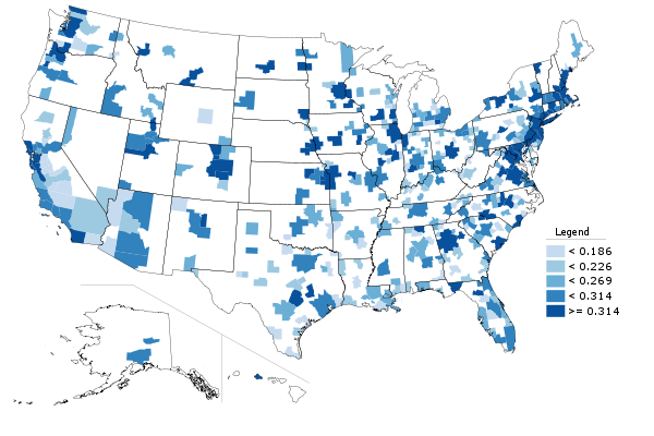
    Metro area college degree attainment, 2010

    I’m going to roll out a series of posts covering the highlights of some of this data. I’ll start with educational attainment, since that is something that is so key to upward social mobility and urban economic success.

    But first I’ll put in a brief plug for my Telestrian tool. The Census Bureau site for distributing this data is a disaster. As one Brookings senior fellow put it, “Lots of Census data yesterday, today. Lots of angles, stories, conclusions. One shared sentiment: new American Factfinder is AWFUL” and “New Factfinder making mainframe punchcards look appealing.” Telestrian is designed for very rapid basic analysis and comparative benchmarking moreso than simple fact lookups (though it can do that do). In fact, I generated every table, graph and map in this post in ten total minutes with it. Even if you aren’t in the market for a commercial product, there’s a no credit card required free trial period, so if you are interested in perusing the ACS data and don’t want to beat your head against the wall with the Census Factfinder, I encourage you to check it out. Telestrian doesn’t have every data element, but it has a lot of interesting stuff.

    College Degree Attainment

    College degree attainment (the percentage of adults with a bachelors degree or higher), is one of the most critical factors in urban success. If you’d like to know more, just check out all the great research on it under the heading of “talent dividend” over at CEOs for Cities.

    The map at the top of the post is 2010 college degree attainment for metro areas. Here are the top ten, among those with a population greater than one million, showing total number of people with degrees and the attainment percentage:


    Row Metro Area 2010
    1 Washington-Arlington-Alexandria, DC-VA-MD-WV 1,758,297 (46.8%)
    2 San Jose-Sunnyvale-Santa Clara, CA 558,519 (45.3%)
    3 San Francisco-Oakland-Fremont, CA 1,317,354 (43.4%)
    4 Boston-Cambridge-Quincy, MA-NH 1,335,276 (43.0%)
    5 Raleigh-Cary, NC 301,012 (41.0%)
    6 Austin-Round Rock-San Marcos, TX 429,163 (39.4%)
    7 Denver-Aurora-Broomfield, CO 651,661 (38.2%)
    8 Minneapolis-St. Paul-Bloomington, MN-WI 822,321 (37.9%)
    9 Seattle-Tacoma-Bellevue, WA 867,193 (37.0%)
    10 New York-Northern New Jersey-Long Island, NY-NJ-PA 4,613,445 (36.0%)

    And here’s the bottom ten:


    Row Metro Area 2010
    1 Riverside-San Bernardino-Ontario, CA 499,663 (19.5%)
    2 Las Vegas-Paradise, NV 278,387 (21.6%)
    3 Memphis, TN-MS-AR 209,987 (25.1%)
    4 San Antonio-New Braunfels, TX 344,247 (25.4%)
    5 Louisville/Jefferson County, KY-IN 224,392 (25.8%)
    6 Tampa-St. Petersburg-Clearwater, FL 513,182 (26.2%)
    7 Birmingham-Hoover, AL 198,856 (26.3%)
    8 New Orleans-Metairie-Kenner, LA 209,916 (26.8%)
    9 Jacksonville, FL 241,801 (26.9%)
    10 Phoenix-Mesa-Glendale, AZ 731,643 (27.2%)

    While we are on the topic, here is a map of college degree attainment by state:


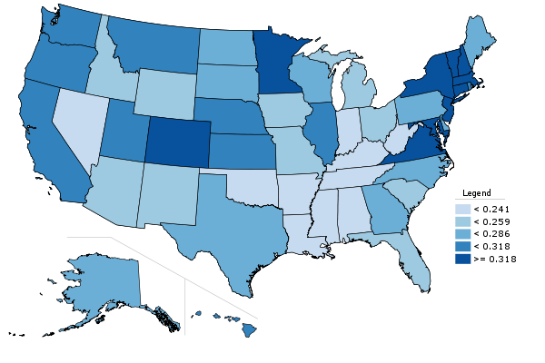
    State college degree attainment, 2010

    And here is county level college degree attainment for those counties covered by the 1-year ACS:


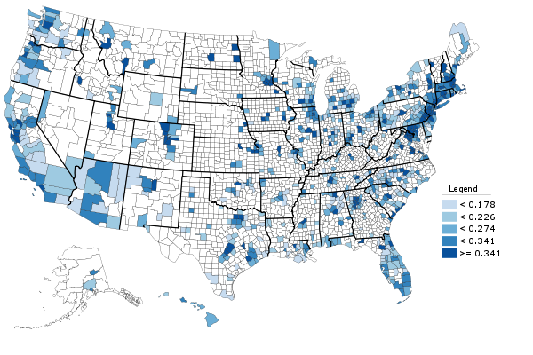
    County college degree attainment, 2010

    Changes in College Degree Attainment

    Beyond just the raw 2010 numbers, it’s interesting to look at which places are growing their college degree attainment the most. That is, which places are growing their talent base. So here’s a look at metros by their change in college degree attainment over the last decade:


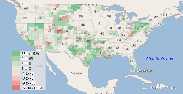
    Change in percentage of adults with college degrees, 2000-2010.

    Some places already have very high college degree attainment, which can make it tougher to grow even higher. Speaking of which, the US as a whole raised its college degree attainment as well. To some extent, this is purely a function of demographics. Older generations have lower educational levels than younger ones. (None of my grandparents had a college degree, and my father’s parents never even finished high school. I don’t think that was atypical for their day).

    What might be more interesting to look at is whether places are increasing their college degree attainment faster or slower than the US overall. There’s a measure that does capture that. It’s called location quotient, and is used in economic analysis to measure the concentration of industries in certain locations.

    An economist told me once that he likes to look at this for all sorts of things, not just industry clusters. The formula works for other stuff. I really haven’t seen this used before, so caveat emptor, but here’s a look at shifts in location quotient for metro areas over the course of the decade:


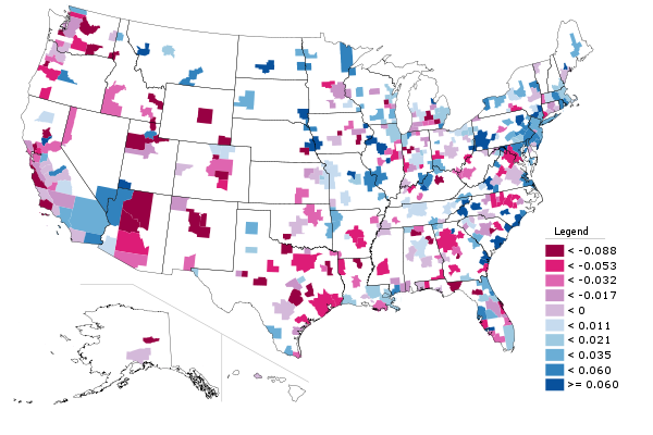
    Metro area change in location quotient for college degree attainment, 2000-2010. Increase in LQ in blue, decrease in red.

    The blue metro areas had a higher concentration of college degrees relative to the nation as a whole in 2010 than they did in 2000. The red ones a lower concentration. This is certainly an interesting area for further exploration.

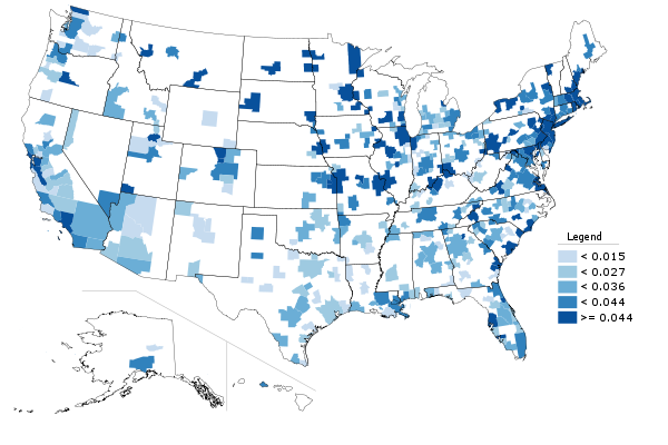
    While I’m on the topic, here’s the same chart, only limited to graduate and professional degrees. There’s some interesting variability here.


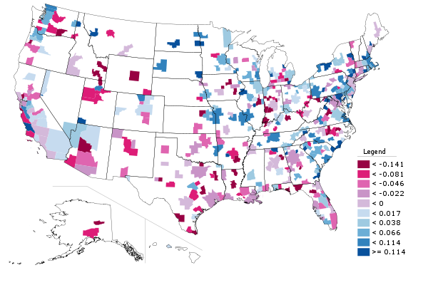
    Metro area change in location quotient for graduate and professional degree attainment, 2000-2010. Increase in LQ in blue, decrease in red.

    A Closer Look at Indianapolis

    Just as one more granular example, I wanted to take a look at the Indianapolis vertical. Here’s 2010 college degree attainment for the city, metro, state, and America as a whole:


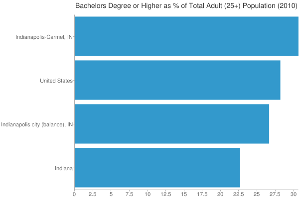
    College degree attainment, 2010

    As we know, urban regions tend to be more highly educated. Here we see that while Indiana is one of the lowest states in terms of college degree attainment, the Indy metro area actually beats the US average. However, the city of Indianapolis falls short of the US average. Because Indy is a consolidated city-county government that includes a lot of inner ring suburban areas, it’s hard to draw conclusions about the true urban core, but it does seem clear that the center is less educated than the periphery of the metro.

    Now lets look at the change in attainment for the decade:


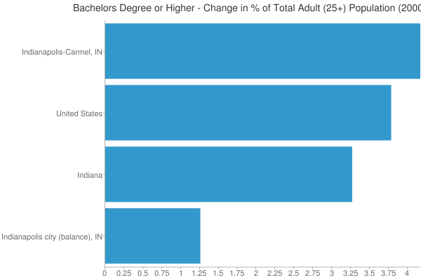
    Change in the percentage of adults with a college degree, 2000-2010.

    Here we see that the rich get richer, as Indy metro not only started out on a higher base, but had the best showing in attainment growth as well. OTOH, going back to our LQ measure, Indiana actually boosted its LQ while the Indy region was stagnant. That’s because this is a percentage point change, not a percentage change, and growing from a low base makes it easier to boost LQ. It’s one of the quirks of that formula.

    The poor showing of the city of Indianapolis is something that should definitely be worrying. It would be interesting to do a similar analysis for other metros, but alas that’s all for today.

    Aaron M. Renn is an independent writer on urban affairs based in the Midwest. His writings appear at The Urbanophile, where this piece originally appeared. Telestrian was used to analyze data and to create charts for this piece.

  • Are 20th Century Models Relevant to 21st Century Urbanization?

    Analysis of the state of the world’s cities 2010/2011 by UN-Habitat focused on the narrowing urban divide, with 227 million people moving out of slum conditions over the preceding decade.  While acknowledging uncertainty over cause and effect, the report notes that:

    urbanization … is associated in some places with numerous, positive outcomes such as technological innovation, forms of creativity, economic progress, higher standards of living, enhanced democratic accountability and women’s empowerment. … the report calls for policy-makers and planners to understand that urbanization can be a positive force for economic development, leading to desirable social and political outcomes.

    The North Atlantic solution

    The report acknowledges the diversity of urbanisation[1], making its authors’ somewhat singular approach to managing it (more density) incongruous.  Their prescription is based on resisting urban sprawl, reflecting the experience of North America.  They also suggest that sprawl is a sign of “divided cities”, translating into

    an increase in the cost of transport, public infrastructure and of residential and commercial development. Moreover, sprawling metropolitan areas require more energy, metal, concrete and asphalt than do compact cities because homes, offices and utilities are set farther apart.

    The report denounces sprawl in suburban zones of high and middle income groups and in extensive slums on the city edge.  On the latter, they invoke issues of governance, saying it occurs because

    authorities pay little attention to slums, land, services and transport. Authorities lack the ability to predict urban growth and, as a result, fail to provide land for the urbanizing poor.

    Can one size fit all?

    It is difficult to accept prescription predisposed to a particular view. Urbanisation is not a single condition. Differences in the stage of urbanisation, vastly different physical, cultural and economic settings of “urban” settlement, and different institutional arrangements belie the idea of a universal response or that any particular form is best for all cities. 

    Apart from anything else, “western” cities [2] don’t really feature in 21st century urbanism.  Consider the figures.  In 1950 western cities accounted for 43% of the world’s urban population.  This was down to 23% in 1990 and 18% in 2010. UN projections have the figure down to 15% in 2030, accounting for between just 3% and 4% of all urban growth between now and then.

    What Size City?

    This post looks at some more numbers that help illustrate the diversity of urbanisation – the size of urban settlements. 

    According to UN figures,  8% of the world’s population lives in 53 cities housing over 5 million people; 12% in 388 cities of between 1 and 5 million; and 31% in cities of under 1 million. Any prescriptions for urban governance and urban form need to reflect quite extreme divergence between the few megacities and the many smaller settlements where the majority of urbanites live.

    The Urban Growth Trajectory

    Urbanisation experiences vary, also.  The different national experiences of the past 60 years can be illustrated using ten quite different countries (Chart 1).  By 2010, Brazil, US, UK, Mexico, and Iran were all heavily urbanised.  But the level of urbanisation changed little for the US and the UK over thelate 20th century, while it grew rapidly in the others.

    In yet another trajectory, erstwhile rapid urbanisation in Russia stalled after the mid 1980s. 


    Chart 1: Urbanisation Trends, Selected Nations, 1950-2010

    Urbanisation is accelerating in China, but has flattened off in Indonesia.  It has been increasing steadily in Nigeria and slowly but still steadily in India.

    Most people moving into smaller cities

    Chart 2 shows shares of growth by city size groups over the last twenty years. (Russia is omitted because urbanisation actually declined by 5.5%.) 

    Cities of under 1 million residents dominate gains, strongly favouring developing countries.  They accounted for 90% of urban growth in Indonesia, 71% in Nigeria and 66% in Iran. 

    US experienced growth more or less across all size categories, although Chicago went from the 7m-8m to the 8m plus category, reducing down the former.

    Chart 2: Where Populations Grew – Cities by Size Category, 1990-2010

    Brazil, China, and Indonesia saw significant growth across the most size groups.  There appears to be a contrast within these countries between the centralising influence of few large cities and dispersed urbanisation in many much smaller settlements.

    (The picture for the UK reflects a gain of around 1 million people in London — to 8.6m — shifting it between categories.  Smaller cities actually accounted for 82% of the net UK gain in urban population, suggesting a duality between the growth of the capital and decentralisation through growth in smaller settlement). 

    So where are the big cities?

    The US has five urban agglomerations with a population of more than 5m, centred on New York, Los Angeles, Chicago, Philadelphia and Detroit (Chart 3).  Compare this with China, with twelve cities of over 5m, and five cities of more than 8 million people (Shanghai, Beijing, Chongqing, Shenzhen, and Guangzhou); or India, with eight over 5m and three over 8m (Mumbai, Kolkata, and Chennai).

    At the same time, China has 90 cities of between 750,000 and 2m, India 44 and the US 66.  Mexico has 15, Russia 14 and Brazil 13. 

    Chart 3: Number of Cities by Size Category, Ten Nations 2010

    Primacy – a mixed picture

    Single centres that dominate national populations are termed “primate”.  Their rise and fall may be symptomatic of national economic fortunes.  Excessive primacy may increase economic volatility because the contrast between a rich centre and poor periphery is politically destabilising. One centre dominating financial, human, and intellectual resources may also increase national vulnerability to structural decline.

    The picture is mixed across our sample (Chart 4).  Mexico City and London stand out.  High levels of primacy are also evident in Iran and Indonesia, but have been easing, contrasting with Nigeria where it is increasing.  It is least pronounced in the countries with the largest urban populations – China and India — suggesting a strong population pull from a number of state or provincial capitals, as well as a host of much smaller cities.

    Chart 4: Population Share of Largest City, Ten Nations, 1990 and 2010

    So what does all this mean?

    The data confirms huge diversity in the sizes of cities people live in across and within nations.  It generates more questions than answers, though, the main one being whether it is relevant simply to transfer urban governance, management, or planning models from one place to another.  Apart from contrasts within and between nations, it is clear that the west is no longer the focus of urbanisation and is unlikely to hold many of the answers to today’s urban growth challenges.

    The evidence also indicates a tendency for urbanisation to take place in small, dispersed settlements rather than mega-cities.  More modest scale makes different demands on infrastructure and institutions.  It may also help manage urbanisation and ensure that benefits can be better accessed by larger numbers of people.  Small cities, sub-centres in large cities, and districts of modest scale may be better suited to adaptable and innovative planning and management than large scale, extensive cities with their more centralised, remote, and inevitably bureaucratic political and administrative systems. 

    Very large agglomerations do exist, even if they are not as dominant in the wider urban picture as their size and profiles might suggest.  The question they raise is whether they should continue to dominate national and international agenda for urban growth and management.  Dispersed urbanisation may better reflect the resources and capacities needed to support an exploding urban population in the 21st century.

    Phil McDermott is a Director of CityScope Consultants in Auckland, New Zealand, and Adjunct Professor of Regional and Urban Development at Auckland University of Technology.  He works in urban, economic and transport development throughout New Zealand and in Australia, Asia, and the Pacific.  He was formerly Head of the School of Resource and Environmental Planning at Massey University and General Manager of the Centre for Asia Pacific Aviation in Sydney. This piece originally appeared at is blog: Cities Matter.


    [1]  The lowest level of urbanisation incorporated by the UN depends on the conventions of individual nations but may refer to settlements with as few as 2,000 people.

    [2] Treated here as North America, Northern Western and Southern Europe, and Australasia

    Photo by NASA’s Marshall Space Flight Center.

  • What Boomers Are Choosing

    In 1989, a man came to my office and introduced himself as the vice president of development for the Del Webb Corporation.  He retained my firm to prepare a master plan for their first active-adult community outside of their typical desert southwest market. 

    This led me to an exploration of what made a successful active adult community.  I learned they required unique and distinct considerations quite different from those used in more conventional master planned communities.  During the information gathering process, I toured each of the Sun City projects, interviewing staff and visiting residents to understand the qualities and features which attracted buyers and provided the lifestyle sought by retirees. 

    Since that initial project, I and my partners have had the opportunity to plan and design over 60 active adult communities, many of which were realized and built out over the past 10 years.  We have also worked with existing active adult communities to expand or enhance their amenities and programming to remain relevant to the changing needs of the boomer resident and buyer.

    Over the past several years, our firm began working with small towns and rural communities utilizing our insight and knowledge of the retiree market and desired community amenities to create or enhance their position as a retirement destination.  Additionally, we have assisted them in establishing programs to recruit retirees as an economic development strategy that taps into economic, social, educational and professional attributes of the boomers. 

    Through my work with both the active adult and rural/small town communities I have observed changing trends in the retiree market as the Eisenhower generation gave way to the boomers.  The following are some of the patterns and behaviors which are vital to the boomer home buyer as they make decisions on their retirement living.

    Trend 1 – When making a decision regarding retirement housing, boomers are savvy consumers, typically having purchased between 3 – 9 homes in their lifetime.  These are buyers who know what they want and are reluctant to compromise their selection criteria.

    Trend 2 – Recreation preferences have shifted significantly over the 35 years I have worked in this market.  In the late 80s, virtually all active adult communities relied on golf as the primary community amenity.  Now golf ranks 8th as the preferred amenity of retirees and continues to decline in popularity.  Walking facilities are by far the most requested amenity in retiree focus groups followed by fishing, bocce, tennis and pickleball.

    Trend 3 – The preferred design of single family homes sought by retirees remains one-story living with no steps between parking and front door.  The size of individual dwellings is smaller but still well constructed and featuring no reduction in amenities.  However, specialty rooms are being replaced by multi-use space.  My favorite analogy is the comparison of a Cadillac to a BMW.  There is also increased demand for design and construction techniques which enhance the conservation of water, electricity and natural gas.

    Trend 4 – Community size is smaller, ranging from 10,000 to 2,500 units.  The trend now reflects a growing demand in the market for smaller, more intimate communities.  Finance and entitlement issues further support this trend.

    Trend 5 – 65% of boomers desire to continue their education through formal and informal means during retirement.  This preference drives the decision to purchase a home in towns with a college or an established academic program.  Communities which do not have higher learning institutions have brought in private education, on-line and community educational entities.  Senior University in Georgetown, Texas was established to meet this demand by the residents of Sun City Texas.

    Trend 6 – Historic residential sales patterns show that the “resort-style active adult community” appeals to only 7% of the age and income qualified boomer market.  Small towns and rural locations, however, are finding themselves the preferred destination for boomers in retirement.

    Trend 7 – We know there are many factors which are essential to attracting retirees including affordability, health care, transportation, established social fabric, significant retention of visual history and moderate climate.  However, there is a much greater emphasis on proximity to family, especially grandchildren.  This is driving the relocation decision for many boomers.  Additionally, safety and security have been identified by a greater portion of focus group participants. This preference has become more difficult to realize due to a growing reluctance by municipalities to allow private roads and secure entry gates as a facet of the community’s security program.  The requirement for connectivity is also complicating this trend.

    Trend 8 – Boomers are not flocking en masse to multi-family dwellings in urban cores.  Robert Charles Lesser and Company recently reported that only 4% of affluent empty nesters indicated they would move to a condo downtown in their current metro area while 3% would chose a condo in a suburb of their current metro area.  Essentially, there is little migration of retirees from rural communities and the suburbs to the urban core, contrary to widely held beliefs.

    Overall, the boomer market is diverse and no one solution will appeal to the entire market.  A knowledgeable developer or small town councilman must formulate their plans on local preferences and values.  And remember that many of the myths perpetuated by the media – notably the return en masse of boomers into the city – are just that, a myth.

    Joe Verdoorn, a Principal at SEC Planning, LLC, has over 40 years land planning and development experience working with clients such as Pulte/Del Webb, Motorola, Apple and Hunt Investments.  He is a pioneer in the field of active adult community design who continues to research the retiree market to understand their evolving wants and needs. 

  • The Ambiguous Triumph of the “Urban Age”

    In its State of the Population report in 2007, the United Nations Population Fund made this ringing declaration:  “In 2008, the world reaches an invisible but momentous milestone: For the first time in history, more than half its human population, 3.3 billion people, will be living in urban areas.”

    The agency’s voice was one of many trumpeting an epoch-making event.  For the last several years, newspaper and magazine articles, television shows and scholarly papers have explored the premise that  because most of the world now lives in urban rather than in rural areas things are going to be, or at least should be, different.  Often the conclusion is that cities may finally get the attention they deserve from policy makers and governments.  This optimism dovetails nicely with a sizeable literature of urban advocacy chronicling the rejuvenation of central cities and extolling the supposed virtues of high-density city living, even predicting the withering away of the suburbs.

    This supposed triumph of the urban is fraught with ironies, however.   The first is that, rather than a simple rush of people from the hinterlands into the centers of high density cities, there has also been, within almost every urban area in the world, a significant move of the population outward, from dense city centers into peripheral suburban areas and beyond them into very low-density exurban regions.   

    We can use Paris as a typical example.  The city of Paris reached its peak population of nearly 3 million in the 1920s.  It has lost nearly a third of its population since then.  What remains in the city is a smaller and wealthier population.  At the same time the suburbs, accommodating both families of modest income forced out of the city as well as a burgeoning middle class,  have grown enormously, from two million to over eight million.  And this does not count a great deal of essentially urban population that that lives in a vast ring of exurban or “peri-urban” settlement.  Certainly the majority of “urban” dwellers in the Paris region do not live in the elegant apartment blocks along the great boulevards familiar to the tourist.   They live in houses or small apartment buildings in the suburbs and use the automobile for their daily transportation needs.

    In fact, Paris is a good example of an even more fundamental irony.  At the very moment when urban population has been reported to surpass the rural, this distinction has lost most of its significance, at least in many parts of the affluent world.  Two hundred years ago, before automobiles, telephones, the internet and express package services,  cities were much more compact and rural life was indeed very different from urban life.  Most inhabitants of rural areas were tied to agriculture or industries devoted to the extraction of natural resources. Their lives were fundamentally different from those of urban dwellers. 

    Today the situation has changed radically.  Most people living in areas classified as rural don’t farm or have any direct connection with agriculture.  They hold jobs similar to those in urban areas.  And although they might not have opera houses, upscale boutiques or specialized hospitals nearby, the activities that take place in these venues are available to them in ways that they never were before.

    I can confirm the way the distinction between urban and rural has broken down by looking out the window of the house in Omro, WI where I am staying this weekend.  Omro, population about 3000, is located 8 miles west of Oshkosh and is  legally a city under Wisconsin law.  It is also an “urban” place according to the Census Bureau which, like those of other countries, defines urban largely by density standards.   In the case of the US, this means, in simplest terms, a density of at least 1000 people per square mile or just under two people per acre. 

    At one time this 1000-people-per-square-mile figure did provide a logical demarcation line.  Above those densities were places that could afford urban services like public water and sewers, sidewalks, streetlights, municipal fire departments and libraries.  Below that level were places that either didn’t have these services or had to depend on faraway county governments.  Unless you were closely associated with agricultural production or other rural economic activities or you were wealthy enough to provide your own services, it was quite inconvenient to live in rural areas. 

    Today, the automobile, rural electrification, the internet and the rise of alternate and privatized services has transformed what it means to live in rural areas.  “Country living” today has few of the drawbacks that made it inconvenient for middle class residents as recently as fifty years ago, and the migration of so many urbanites into the country has blurred the distinction between urban and rural.

    The view out my window bears this out.  When I look one direction what I see are city streets and houses on land that is technically urban.  Of course, Omro, with a single main street, two traffic lights and only a handful of stores, is not at all the kind of place that most people associate with the words “city” or “urban.”  Like the majority of small urban places in this country, its densities are lower than those found in the suburbs of larger cities.   When I look out the other direction I see mostly fields beyond the city limit.  But, unlike the case in the past,  there is no sharp divide.  There has been a significant increase in the number of houses out in the area that is technically “rural.”  Some of these used to be farmhouses, but there are few farmers anywhere for miles around.  Most farming is now done under contract or  as a large industrial-scale operation.   

    Most of the houses in the “rural” area around Omro have been built in the last decade or two and never housed anyone with any direct connection to farming.  They are suburban in appearance and mostly inhabited by people who work at home, are retired or commute some distance to jobs spread across a vast swath of urban territory that stretches from Fond du Lac south of Lake Winnebago to Green Bay where the Fox River meets Lake Michigan. 

    The result is that today, as you drive outward from the center of Fond du Lac, Oshkosh, Appleton or Green Bay, the number of houses per square mile diminishes, but there is no clear break between city and country.  It is a crazy quilt of agricultural, residential and other uses.  Commuting patterns, if charted on a map, would form a giant matrix of lines running in all directions.  Whether one is in the center of Oshkosh or 50 miles away, however, one can still live an essentially urban existence.   

    This same diffused urban condition holds true for very large swaths of the United States wherever there is enough underground water to allow wells. It is particularly conspicuous in the older and more densely settled eastern part of the country.  A state like New Jersey exhibits a pattern of dense older cities, radiating suburbs, vast exurban territories and farmland and open space, overlapping in ways that confound traditional notions about what is urban and rural. In places like New Jersey, the census distinction has lost almost all of its meaning.

    I don’t mean to suggest that that the news that the majority of the world’s population is now urban has no significance.  In fact this move from the countryside to urban areas has been one of the defining events of world history over the last several centuries.  Although this process was mostly finished in Western Europe and the United States decades ago, it still continues in most of Latin America, Africa and Asia and accounts for a great deal of the dramatic upward surge in income throughout the world.

    Nor am I suggesting the demise of the great cities of Europe or America.  Far from it.  Many rich families in particular will probably continue to choose high-density neighborhoods like those on the Upper East Side of New York or the 16th arrondissement in Paris, although often with a rural retreat as well  As the world gets wealthier, more people may make a choice to live in this way.

    However, current trends give no reason to believe that places like Manhattan or central Paris are going to increase in population and density as part of a “back-to-the-city” movement.    As cities gentrify, they undoubtedly become more attractive, but increased demand leads to higher prices keeping out many families who might choose to live in them.  Furthermore, the gentrifiers tend to have smaller families than those they replace, and they also tend to demand  more room, larger and better equipped housing units, more parks and open spaces.  Because of this, the gentrifiers, citing the need to preserve existing neighborhoods, frequently put up all kinds of barriers to new development and increased population and density, particularly by less affluent citizens.  For all these reasons,  existing city centers in the affluent world are unlikely to accommodate a significantly larger percentage of the population.

    Even in the developing countries, as urbanist Shlomo Angel has shown, most cities are spreading outward at ever lower overall densities just as cities have been doing for many years in the affluent West. For those who don’t have a lot of affluence, and even some who do, low density suburban- and increasingly, even lower density exurban- living, remains alluring for many in both the affluent and the developing world.   In fact, we might even be seeing the initial stages of a major reversal of the kind of urbanization that characterized industrializing cities in the West in the 19th and early 20th centuries. The sharp increase in houses outside Omro may presage at least a partial return to a pre-industrial condition seen, for example, in nineteenth century America when people were more evenly spread across the landscape. 

    This continuing urban sprawl is, of course, deplored by many of those who celebrate the supposed triumph of the “urban age. “ Yet  as I have argued in my book Sprawl:  A Compact History, this phenomenon is by no means as bad as most anti-sprawl crusaders imagine it to be.  Continuing to spread the population could conceivably result in a more equitable, more sustainable pattern of living, particularly as renewable energy and other resources are harvested close to home with less need of the giant systems necessary to maintain our dense industrial-age cities.  In any case, despite all of the planning regulations put in place in cities throughout the affluent world to control growth at the edge, the periphery continues, inexorably, to expand almost everywhere. 

    Nowhere does the evidence suggest that we are witnessing the final triumph of the traditional high-density city.  In fact, the much-ballyhooed urban majority might be in great part a statistical artifact, a way of counting the population that over-emphasizes the move from country to city and fails to account for the powerful counter-movement from the city back toward the countryside.  Indeed the emerging reality of overlapping patterns of high density centers, lower-density peripheries and vast areas of very low density urban settlement, all of them interspersed with agricultural lands and protected open spaces, threatens to upend altogether the traditional notion of what it means to be urban.   

    Robert Bruegmann is professor emeritus of Art history, Architecture and Urban Planning at the University of Illinois at Chicago.

    Photo by urbanfeel.

  • Commercial Real Estate: Shrinking to Fit

    We are going to need less commercial real estate in the future, at least on a per-unit-of-population basis. Advances in communications technology are causing profound and sometimes unanticipated changes in our lives.

    Retail Markets
    The coming change is most obvious in retail markets. Americans are increasingly shopping online. However, we’ve really just started to scratch the surface. According to the U.S. Census Bureau’s 2009 E-Stats report issued in May, 2011, E-commerce only accounted for 3.99 percent of U.S. retail sales in 2009.

    I was surprised at how small that number was. Certainly it is higher now, and the 2009 number was almost double 2004’s 2.13 percent, but there is huge room for increased internet retail sales. This is a growth business with a capital G.

    Originally, I believed that traditional brick-and-mortar retailers would have the advantages of customer service and product knowledge, and internet purchasers would be product-savvy shoppers looking for products that they already knew about. That has turned out not be the case at all.

    It is true that the initial internet retail sales successes have been in products where technical knowledge is not critical, and tastes are well established; products such as music, movies, and books. However, online retailers have made impressive gains in providing customer assistance to shoppers looking for more technical products.

    Ratings of products and retailers were an initial step, along with detailed technical data. More recently, internet retailers have added chat windows, some with pictures of the salesperson. It won’t be long until voice or live video are offered, if it isn’t already.

    It is now the case that you are more likely to find more informed assistance on the internet than you will from a brick-and-mortar retailer. This is not to say you can’t find good assistance at a traditional retailer. But your online experience is likely to be better than what you will receive if you walk into a store and deal with the first person you bump into.

    As internet sales increase, expect to see fewer traditional retailers and less demand for retail space. Already, shopping centers anchored by a music store, a video store, or a book store have felt the impacts. This is only the beginning.

    Commercial rents will be softer and vacancies higher in large regional centers and in neighborhood strip malls. This will tend to drive retailers to ever larger centers with more traffic. Smaller centers will likely slowly deteriorate and die. In the end, we’ll have fewer retail centers, but the average center will be larger than it is today.

    Office Markets
    While the number of workers telecommuting is still small, it is growing; someday, it will be very large. Initially, the growth in telecommuting was driven by workers’ desires to physically commute on fewer days. Today, the initiative is changing to employers.

    Companies that adapted to telecommuting employees began to learn how to supervise these workers. Some companies have gone further. My son works for a company that has closed many physical offices, but kept most employees. Everyone was told to telecommute.

    For companies that have made the strategic decision to reduce office space, the advantages must be large. Certainly rent goes down, but other expenses go down too. Heating and cooling costs go away. The company no longer needs to support a local network, with the local network’s support costs.

    I haven’t seen research on telecommuters’ productivity, but it is easy to imagine it increases. Think “happy employees are productive employees.” It is also easy to imagine that productivity decreases. Think “unsupervised employees are unproductive employees.” Clearly, telecommuter productivity is the key to profitably running an office-free operation. As someone once said “any job performed on a computer can be performed anywhere.”

    The lower demand will result in lower office space rental prices and higher vacancies. Again, this should lead to office-dependent operations migrating to the better addresses. In the end, the less-desirable buildings will be empty.

    Industrial Markets
    We’ve seen the huge increase in overseas manufacturing, and we’ve seen the steady decline of U.S. manufacturing jobs. That is just the first stage of a profound transformation in the way things are produced. As the song goes., “You ain’t seen nothing yet.”

    Manufacturing’s future is nicely exemplified by three-dimensional printing. Today, you can Google “three dimensional printing” to find links to videos of three-dimensional printers producing amazingly complicated products, or find companies that have three-dimensional printers. Or you can use a three-dimensional printer to produce something.

    I expect the growth of three-dimensional printers to be something like what we saw with copy machines. The first copy machine I used was in a drug store, and it was coin operated. Then, the banks made them available to customers. Today, we all have at least one in our home and one at the office.

    The day will come when three-dimensional printers will be ubiquitous. You will download instructions for products from some company like Amazon. Then you will produce your good, without the need for an industrial building or a brick and mortar retailer. Producers of products that can’t be printed will print parts, reducing the demand for other producers, inventories, and shipping.

    Any Growth Areas?
    Buildings associated with providing healthcare may be the major exception to declining commercial real estate demand. The aging population, new technology, and long-term wealth trends are likely to continue to drive growth in the economy’s only sector that has grown consistently throughout the recession. At least so far, technological advances in medical care have increased demand for space instead of decreasing it.

    Specialized R&D space may also buck the trend. Many of these facilities can be specialized, however, to the point of being profitably used by only one company. That implies that these buildings are risky investments.

    Policy Implications
    The decline in commercial real estate demand will pose serious challenges to governments. We’re already seeing states and local governments struggle with loss in retail taxes from internet sales . Declining revenues are just the beginning, though. Expenses will increase.

    Empty buildings generate crime. In the case of retail centers, the crime will be very public. Nearby residential property values could decrease, with additional lost revenue to governments. Residents will not stand idly by. They will demand effective action — action that could be very expensive.

    To minimize the fiscal damage, local governments will need to be nimble, a characteristic that few governments possess. They will need to be willing to change zoning codes to adapt to the decline in commercial real estate. They need to allow owners of existing space to redevelop or change their product mix. They may need special tax districts to deal with the blight created by vacant properties.

    Growing population and an eventual real recovery will eventually fix the residential real estate problem. Commercial real estate’s challenges will not be so easily addressed. The impacts are not only on owners, developers, and contractors . All of us will be affected. The time to plan for those changes is now.

    Bill Watkins is a professor at California Lutheran University and runs the Center for Economic Research and Forecasting, which can be found at clucerf.org

    Photo by Mark Lyon — Full Floor For Rent.

  • Queensland’s Future: Diverse and Dispersed

    I was recently asked to outline my thoughts on how the Queensland urban landscape might look 40 to 50 years from now.  Go on, you can laugh.  I did too.  It’s hard enough to forecast the next 12 months, let alone two generations away, but I’ve given it a go, of sorts, so here it is:

    First though, it might be best to outline my methodology.  In short, this forecast will be based on underlying trends, some understanding of human nature, and importantly, the Australian mindset.  My outlook is supported by evidence – what people actually do rather than say – and importantly, not by urban myths or fallacies, despite the frequency with which they have been aired of late.  Unfortunately, we don’t have the space or the time here to support every claim or go into massive detail; so this discussion is confined to broad shapes – not nitty gritty.

    Queensland’s urban future (and that of Australia) can best be summed up in two words – Diverse and Dispersed.

    Let’s deal with the second D – dispersion – first.  Our regional centres are likely to become a whole lot bigger and at the expense of the already crowded south-east corner of the state.  The move away from the world’s bigger cities is already underway, as evidenced in the recent census in the United States, but also throughout much of Europe.  Several Asian and Middle-eastern countries are now also following suite  As a Mckinsey Institute study recently found, smaller cities, particularly in the developing world, are growing considerably faster than the much discussed megacities.

    The annual ABS small-area population data suggests this trend is also very true in Australia and particularly in Queensland, which, over the past decade, been the fastest growing state on the continent, appears to be following the same trend, something likely to be borne out by 2011 Census, due later this year .

    Within our capital cities themselves, the much ballyhooed move downtown will slow – again, it already is doing so – as the cost to live within close proximity to the CBD is just too high compared to the real benefits. 

    The irrational assertions about the trend towards denser living rest on urban myths that promote inner city density over other housing forms. These include the notion that suburban growth worsens carbon emissions and traffic congestion; people are being forced to live far from jobs concentrated in our CBDs and denser development will make it cheaper for them to get to work. These notions are all largely exaggerated or incorrect. More to the point, they stand in opposition to the basic preferences of the market.  

    Instead of having a single high-density city core, with lower development density radiating outwards, the most likely urban shape in the future will be one of more even distribution of housing density throughout the city; concentrated more, no doubt, around middle-ring transport hubs and new master planned town-centres.  Our middle-ring and outer suburbs will have much more compact urban settings but will remain primarily dominated by relatively low density housing.

    Diversity relates to the housing stock itself.  The current push towards smaller dwellings has little to do with demographics and the market’s wants, but reflects basic reaction to diminished housing affordability.   There is a demand for tightly-sized product, but it is nowhere as near as high, nor is the long-term trend towards such as strong, as the urban boosters advocate.

    Taking a wider view, Australia (and America too) is still in its frontier or "barbaric" stage of its cultural evolution.  We walk with wide gaits, worship most things large from roadside bananas to women’s appendages, and don’t really like crowded spaces or queues Most of us like our space; aren’t really ready to give it up, and are not likely to do so for many decades to come.

    Rather than remaining focused on density and concentration, it could well serve the community to focus on what appeals to the vast majority of the population, particularly the middle and working class families.  A more practical approach might be to foster the development of smaller, more efficient cities, as well as expansive suburbs and revived small towns rather than engage in a manic drive towards persistent centralization. 

    Rather a forced density agenda on a largely unwilling population, it makes sense to consider how to make a more dispersed (and diverse) urban future more workable and sustainable. Innovations in work environments, notably increased use of telecommuting and dispersed workplaces, and more fuel efficient cars hold more promise than plans that force Aussies to live a way the vast majority do not prefer.

    This article originally appeared in the June/July 2011 edition of the UDIA Queensland’s Urban Developer Magazine.

    Michael Matusik is a qualified town planner and director of independent residential development advisory firm, Matusik Property Insights.

    Photo by Michael Zimmer.

  • Permeable Pavement: Looking Below The Surface

    How can we prevent situations where environmental ‘solutions’ end up in failure? The tale of problems encountered with the misuse of pervious pavers (also known as porous or permeable pavers), used as an eco- friendly option, provides some answers.

    Low impact sidewalk and street installations can become economic problems. Why? Because failed environmental solutions placed on public property are then replaced with conventional construction, using tax dollars. The EPA Section 438 mandating all owned and leased Federal Facilities be converted into low impact development promotes permeable pavement, that is, paving that allows rainwater to pour through it, instead of running off at high speed to an inlet and overloading the storm sewer system, taking pollutants downstream with the water, and eventually infecting our streams and oceans. To understand more about it, read reporter Dave Peterson’s exposés in the Minneapolis Star Tribune.

    On the surface, permeable pavers seems logical: pavement that allows rain to fall through. But what happens after the rain falls through the pavement – where does the floodwater go? A sub-base is needed to support the pavement. The rainfall must fall not only through the pavers, but also through the ground below. If you were to place permeable pavers on your back yard patio, supporting the weight of people and furniture would require very little sub-structure. If your lot was made of sandy soil that allows rain to quickly filter through, better yet. But if the ground underneath is clay or rock, the water must be retained or piped off with a sub-drainage system. If this is starting to sound expensive, as we say in Minnesota, you betcha!

    This sub-surface material must be sponge-like, and allow a conduit for water to either pass through to a piped system to be transported elsewhere, or have enough small void areas to retain the water until it can slowly be filtered through its lowest layer seeping back to the earth. To create a ‘base’ with properties that has ‘void spaces’, plenty of rock and large stone is used.

    Of course this means digging a very deep channel under the proposed pavement, moving (removing) the old soil and hauling in this sub-base material. A 100 foot long 30 foot wide road would require a five foot deep excavation with 555 cubic yards of soil to be removed, and almost the same in sub-base to be hauled in. Since a large dump truck holds up to 20 cubic yards (typically less), that small section of street would require at least 27 trips to and from the destination with 27 truckloads of rock, no doubt consuming massive amounts of petroleum.

    Anybody who has been in Minnesota in the winter knows that during, those seven months of freezing weather, cold is redefined. Water expands about nine percent as it freezes, so 555 cubic yards of water would increase about 50 cubic yards. Where does the water go? Up! Water pressure can lift pavers and cause havoc in the winter, so before cold weather sets in it is recommended that the liquid be vacuumed out of the sub-surface and hauled away. Now how much energy does that take?

    People and patio furniture are not that heavy, certainly not as heavy as a bus, which weighs somewhere between 26 and 40 thousand pounds transferred to the tires, depending upon the size and how many it is carrying. This weight is then transferred to the pavement, which is on top of rocks and stone that are intentionally ‘loose,’ to hold water.

    There is another problem with permeable pavement in some applications: water settles to a level surface. A few years ago we designed a low-impact, clustered neighborhood in Minnesota. At the ‘consultants’ meeting with the developer, the young engineer pushed the permeable paver idea. We had designed the neighborhood by harnessing the natural grade, embracing the heavily wooded site’s natural drainage to save most of the existing trees on the steep slopes. In other words, we planned to use what nature provided, eliminating much of the grading, costs and environmental impacts. On this site there were some fairly steep grades, in many cases exceeding a five foot drop in its length along private drives.

    The engineer aggressively insisted on permeable pavers. His idea was to create a five foot deep sub-base under the private drives (26’ wide) and run the gutters of the roofs underground to the sub-surface drainage system. In such meetings it is not polite to scream, “Are you out of your mind?” Instead, after the meeting I told the developer to kill the idea for being far too expensive. The developer did not heed my advice, and when the economics of the engineering was done, the cost escalated out of control. Several months of the engineer trying to (unsuccessfully) convince the city that the permeable pavers was a great solution caused the project to be delayed. By the time it was approved (with the natural drainage solution), the recession was in full swing and the development went dormant.

    From a personal experience, when I built my Green Certified home in 2008, MNGreenstar provided points for permeable pavement but only if the underlying base held the storm water underneath. The soil of my lot is sandy, and could have quickly absorbed the rainwater, allowing a fairly cheap sub-base, but the ‘green’ certification did not allow for compromise. The green certification ‘all or nothing’ approach meant that my sub-surface would have added $5,000 to the construction to get a few green ‘points’ encouraging the ‘nothing’ side of the equation. So, instead of designing the driveway with permeable pavement, we used sculpted landscaped strips (like the driveways of yesterday) to reduce the paved surface area and the overall costs. It is not unusual to see people taking pictures of my ‘low impact’ driveway, which adds curb appeal and value, however, we gained no green points for this logical solution.

    Why the motivation to push permeable pavement? In many cases it might indeed make sense. One reason is profitability, not by those selling the pavement alternatives, but by the consulting industry that specifies materials charging fees based upon a percentage of the construction cost. Permeable pavers and other ‘green’ alternatives can add a considerable amount to costs, and to the profitability of a consulting firm. If all bids were based upon rewarding solutions that cost less, with a penalty for solutions that cost more, consultants would truly deliver on the promise of sustainability; development costs and future maintenance burdens would plummet, while the environment would benefit. If we rewarded engineers employed by government agencies by allowing them to share a percentage of the money they saved by introducing green solutions that are cost effective, it would bring about change overnight.

    Can this be done? Absolutely. The technology and educational materials have been developed for this overhaul, but it would take effort and investment, since we’re currently in an economy where up to 65% of the architectural and land consultants are unemployed, and those remaining are not exactly overloaded with work.

    The EPA Section 438 is the Federal agenda to rebuild existing facilities and have all new construction (including all military bases) comply with low impact standards. On some new construction and redevelopment, permeable pavement could be effective, but it is unlikely to be cost effective where heavy loads, bad soils, and/or frigid weather occur.

    The decreased pavement width of New Urbanism is a start in the right direction, as long as safety and functionality are maintained. Combined with the reduced ‘length’ of infrastructure in plans like Prefurbia, it is entirely possible to reduce the environmental impact of newly paved development by about 30%, and of re-developed areas (i.e. EPA Section 438) by more than 50%, while increasing function and value. Now that we have the knowledge to do so, isn’t it time to start reaping the benefits of design techniques that reduce pavement without harming function?

    Photo by Mockney Rebel; “Pavement Archeology”

    Rick Harrison is President of Rick Harrison Site Design Studio and Neighborhood Innovations, LLC. He is author of Prefurbia: Reinventing The Suburbs From Disdainable To Sustainable and creator of Performance Planning System. His websites are rhsdplanning.com and performanceplanningsystem.com.

  • The Explosion of Oil and Gas Extraction Jobs

    From Appalachia to Alaska, the growth is eye-popping. Thousands of new jobs have sprouted up, most well-paying and all boons to their regions. There’s no denying oil and gas extraction jobs are on the rise, and not just in Texas and Oklahoma.

    North Dakota is drilling oil at a blistering pace. Pennsylvania and West Virginia, along with parts of New York and Ohio, are seeing a natural gas boom with their Marcellus Shale reserves. And Colorado, Wyoming, Alaska, and other Western states are adding extraction jobs in droves.

    The six fastest-growing jobs for 2010-11, according to EMSI’s latest quarterly employment data, are related to oil and gas extraction. This includes service unit operators, derrick operators, rotary drill operators, and roustabouts. Each is expected to grow anywhere from 9% to 11% this year, in an otherwise stagnant economy.

    But that’s not all. A mixed bag of other extraction and petroleum-related jobs—wellhead pumpers, all other extraction workers, geological and petroleum technicians—are also expected to see healthy gains. In total, nine of the top 11 fast-growing jobs in the nation are tied in one way or another to oil and gas extraction.

    Occupation

    2010 Jobs

    2011 Jobs

    Change

    % Change

    Service unit operators, oil, gas, and mining

    42,110

    46,766

    4,656

    11%

    Derrick operators, oil and gas

    23,323

    25,747

    2,424

    10%

    Rotary drill operators, oil and gas

    28,116

    30,981

    2,865

    10%

    Roustabouts, oil and gas

    75,636

    82,678

    7,042

    9%

    Helpers, extraction workers

    44,303

    47,247

    2,944

    7%

    Petroleum engineers

    29,063

    30,917

    1,854

    6%

    Biomedical engineers

    16,065

    17,061

    996

    6%

    Wellhead pumpers

    24,186

    25,616

    1,430

    6%

    Extraction workers, all other

    23,423

    24,784

    1,361

    6%

    Geological and petroleum technicians

    35,304

    37,205

    1,901

    5%

    What’s driving this employment spike? A push for increased domestic oil production is certainly a factor, as are technology breakthroughs in collecting massive shale gas deposits. But more subtle shifts are also happening, including how federal and state agencies track the oil and gas extraction workforce.

    A Prime Example

    For a case study on the skyrocketing employment picture on the shale front, just look at Pennsylvania. Without a tax on natural gas extraction and perfectly located to take advantage of the Marcellus Shale formation, parts of the commonwealth have become a hotbed for drilling. More than 3,000 wells have been drilled in the last three years, and much more is expected in coming years.

    Since 2008, Pennsylvania has added more than 15,000 jobs in the mining, quarrying, and oil and gas extraction industry, a 41% jump. Only Texas and Oklahoma have added more of these jobs in the last three years. Meanwhile, North Dakota has seen an 80% jump in employment in this sector, second only to Delaware since 2008.

    Where are these well-performing oil and gas jobs located? We mapped the data for the four fastest-growing jobs — roustabouts, service unit operators, derrick operators, and rotary drill operators. Here’s what we found: Texas and Oklahoma of course have a large percentage of these jobs, but California, Alaska, and other Western states have a fair share, too.

    The map below shows 2-year job growth in these oil and gas extraction jobs for every county in the continental US. Williams County, North Dakota is No. 1 with 1,539 jobs added, which amounts to 80% growth.

    More Than a One-Year Trend

    Mining, quarrying, and oil and gas extraction is expected to grow 6% in the US from 2010-2011. That’s the fastest projected growth among the 20 broadest-level industries—twice the rate in fact, as the next fastest-growing industry (administrative and support and waste management and remediation services,).

    This is hardly a one-year bump, though. Over the last five years, the explosion in the sector has been than staggering—even with a minor employment dip from 2009-2010. The industry added more than 345,000 jobs nationally from 2007 to 2009, and is expected add another 85,000 this year, which equals 11% growth.

    It’s also helpful to break out mining and oil and gas extraction from the broad sector to more specific industries to locate the real driver of the growth. In this case, it’s easy to see: Of the 506,401 new jobs in the sector since 2006, more than 431,000 have been in the crude petroleum and natural gas extraction industry (NAICS 211111). This sub-sector has grown by a whopping 113% nationally in the last six years while mining (except oil and gas) remains at its ’06 employment level.

    Every state except for Maine has added jobs in crude petroleum and natural gas extraction since 2006, with Texas, Oklahoma, California, and Kansas leading the way.

    The Rise of Contract Oil and Gas Workers

    In last month’s GOVERNING Magazine, William Fulton wrote about the “1099 economy”—the shift by employers to hire temporary workers who file a 1099 form with the IRS rather than a W-2 and don’t receive benefits. No other industry has seen this move to 1099 workers more dramatically than mining, quarrying, and oil and gas extraction.

    A recent EMSI analysis revealed that the share of 1099 workers in this sector increased from 33% in 2005 to 53% in 2010, the biggest percentage jump among the 20 broadest-level industries. Mining, quarrying, and oil, and gas extraction now has the third-highest share of contract workers, behind real estate (74%) and agriculture, forestry, fishing and hunting (68%).

    At least part of this influx could be attributed to land owners cashing in on royalties after leasing their property for drilling. Through the quirks of how the Census’ Bureau of Economic Analysis* tracks the oil and gas extraction industry — and how the industry data is tied to occupations — some of these jobs could be counts of landowners who are claiming additional income from oil and gas royalties. If that’s the case, these jobs would be better placed in the real estate and leasing industry.

    Please note: For these reasons, EMSI “noncovered” data (i.e., data on 1099 workers plus more traditional state data, etc.) for oil and gas jobs should be treated with caution. Also, the jobs numbers for 2010 are estimates at this point, so it will take more time to see how these trends play out.

    *The Bureau of Labor Statistics measures only workers covered by unemployment insurance and who thereby file a W-2. EMSI’s “complete” dataset adds proprietors and other “noncovered” workers by combining BLS and state data with various Census datasets.

    Joshua Wright is an editor at EMSI, an Idaho-based economics firm that provides data and analysis to workforce boards, economic development agencies, higher education institutions, and the private sector. He manages the EMSI blog and is a freelance journalist. Contact him here.

    Lead illustration by Mark Beauchamp.

  • Fifty Years of Population Change in the US: 1960-2010

    A new census leads us to ask how population has changed, but usually discussion is focused on changes since the last census. But even more interesting is to appreciate the vaster changes over a greater sweep of time, for example: the fifty years since 1960, when the United States had 179 million people, toward the end of the post-war Baby Boom.

    Over this fifty year period, the country experienced a tremendous economic expansion and metropolitan growth. The attatched maps and charts display these changes, both in the greatest absolute and relative (percentage) losses and gains. We can then assess areas and regions that changed the most – or the least – and how this pattern differs from the most recent decade.

    Looking at both the maps and the tables, high absolute losses are in large northeastern metropolitan counties, plus, because of Katrina, Orleans (New Orleans).  Next most prominent in terms of losses are mining and small industrial counties in Appalachia as well as the largely rural Black majority counties in the Mississippi delta (Arkansas and Mississippi). Far more widespread in terms of space are small absolutely but often high percentage losses across the Great Plains, the rural small town heartland of the country. Losses do extend to the west, in a few mining and farming counties, as in MT, ID, OR and WA, as well as a few Native American reservation areas. 

    From Table 1 (below), 12 counties lost more than 100,000 people since 1960, most in the northeastern historic urban industrial core, including two New York City boroughs. The bigger loser by far, however, was Wayne (Detroit) . Next were Philadelphia, which lost 477,000 and St. Louis, falling 57 percent from 750,000 to 319,000.   Among non-metropolitan counties, the largest absolute losses were in West Virginia, Kentucky and Pennsylvania (mining), and Arkansas and Mississippi (high Black population).

    High relative losses (table 2) of over 50 percent beset 69 counties, all non-metropolitan   except one: St Louis. States with the greatest number of declining counties included North Dakota, 19; Texas, 16; South Dakota, 6, Kansas, Montana and Nebraska, 4; Arkansas, 3; and Missouri, 2. Most were in the Plains states. It is also clear that a high proportion of counties – both metropolitan and non metropolitan – with high Black populations have experienced losses, a sad commentary on disinvestment in areas with high African-American shares.

    In contrast, the pattern of gains is more complex.  Overwhelmingly, the highest absolute amounts (table 3) – and often percentage gains (table 4) – are in mostly larger metropolitan complexes. For the largest areas, the core counties often had lesser rates of growth, even if the absolute amounts were very large (e.g., Los Angeles, Cook, Dallas-Fort Worth, Houston). In contrast the highest rates of growth, often over 400 percent, took place in their satellite or suburban counties. Most obvious are greater Los Angeles and San Francisco, Denver, the large Texas metropolitan areas, Minneapolis, Chicago-Milwaukee, Atlanta, Indianapolis, Seattle, Portland and Washington, DC.  More recent, less suburban (at least in terms of jurisdiction) dominated areas, often in the Sunbelt, include especially Maricopa (Phoenix), Las Vegas, Salt Lake, Nashville, Charlotte, Raleigh, and Richmond.

    This leaves perhaps the two most spectacular (along with California, obviously: the northeastern Megalopolis and Florida. Florida clearly has the highest overall rate of change over this period. The northeastern Megalopolis is highly varied, but overall now spreading from Richmond, Virginia to Portland, Maine. It has developed into an astounding agglomeration of growth, with the locus of fastest absolute as well as percentage growth in its suburban and exurban portions.

    Growth was also often substantial in non-metropolitan or now small metropolitan areas in many parts of the country. An especially remarkable belt of growth – including small towns – extends from Memphis across Tennessee and North Carolina. Another span of significant growth – despite decline or slower growth in the recent past – lies in the Midwest (Indiana, Ohio, Michigan, Wisconsin and Minnesota). Belts of growth follow the I-5 corridor from California to Canada, the corridor from Tulsa through Fayetteville and Springfield to St Louis, and the I95 coastal south Atlantic strip.

    Sixteen counties gained a million or more: Los Angeles, Orange, San Diego, Riverside and San Bernardino, a southwestern megalopolis; Santa Clara (San Jose); Harris (Houston); Dallas and Fort Worth (Tarrant) and Bexar (San Antonio) in Texas; Miami, Ft. Lauderdale (Broward) and Palm Beach, Florida; Clark (Las Vegas); King (Seattle); and Maricopa (Phoenix).

    Finally the counties which grew at the fastest rate over the 50 years include some 118 that grew by 400 percent or more, and 27 that expanded more than ten-fold. States with the most such counties (400 to 1000 % ) include Florida, 15; Georgia, 11; Colorado, 8; Texas, 6; Virginia 6; California, 4; AZ,MN, MO, NC, and NV, 3 each; MD, NM, OR, TN, WY, 2 each; with 1 each in AL, AR, AK, IL, IN, KY, LA, MS, NE, OK, PA,  SC, UT and WA. Among the over 1000 percent growth, AK and AZ, 1; CO, 3; FL, 8; GA, 4; NV, 2; TX, 6; UT, 1; and VA, 1. 

    Types of counties with over 400 percent growth include 3 core metropolitan, 69 suburban, 44 environmental, and 2 others, often resource development. The fastest growth county was Douglas in suburban Denver, followed by environmentally attractive Mohave, AZ, and Flagler and Collier, FL, followed by Dallas suburb, Collin, and Atlanta suburb Gwinnett.

    Conclusion
    People continue to come to the US in large numbers, and people move from place to place in remarkable numbers.  Don’t count on the current pattern of population to remain very stable, just as the last fifty years have not been.  For example, while the northeastern “Rustbelt” seems in trouble, it is a region of vast plant capacity, superior universities, and a high quality labor force. A reaction to the high cost of excessive outsourcing, and even  some shifts from the “new South” could bring about a surprising restoration.

    Table 1: Largest Absolute Losses, 1960-2010
    Name
    1900
    1960
    2000
    2010
    Change 1960-2010
    Percent Change, 1960-2010
    MI Wayne County 348,793 2,666,297 2,061,162 1,820,584 -845,713 -31.7%
    PA Philadelphia County 1,293,697 2,002,512 1,517,550 1,526,006 -476,506 -23.8%
    MO St. Louis city 575,238 750,026 348,189 319,294 -430,732 -57.4%
    PA Allegheny County 775,058 1,628,587 1,281,666 1,223,348 -405,239 -24.9%
    OH Cuyahoga County 439,120 1,647,895 1,393,978 1,280,122 -367,773 -22.3%
    MD Baltimore city 508,957 939,024 651,154 620,961 -318,063 -33.9%
    LA Orleans Parish 287,104 627,525 484,674 343,829 -283,696 -45.2%
    DC District of Columbia 278,718 763,956 572,059 601,723 -162,233 -21.2%
    NY Erie County 433,686 1,064,688 950,265 919,040 -145,648 -13.7%
    NJ Essex County 359,053 923,545 793,633 783,969 -139,576 -15.1%
    NY Kings County 1,166,582 2,627,319 2,465,326 2,504,700 -122,619 -4.7%
    NY New York County 2,050,600 1,698,281 1,537,195 1,585,873 -112,408 -6.6%
    WI Milwaukee County 330,017 1,036,041 940,164 947,735 -88,306 -8.5%
    MA Suffolk County 611,417 791,329 689,807 722,023 -69,306 -8.8%
    VA Norfolk city 46,624 305,872 234,403 242,803 -63,069 -20.6%
    OH Hamilton County 409,479 864,121 845,303 802,374 -61,747 -7.1%
    OH Mahoning County 70,134 300,480 257,555 238,823 -61,657 -20.5%
    WV Kanawha County 54,696 252,925 200,073 193,063 -59,862 -23.7%
    PA Cambria County 104,837 203,283 152,598 143,679 -59,604 -29.3%
    Table 2: Greatest Relative Losses 1960-2010
    Name
    1900
    1960
    2000
    2010
    Change 1960-2010
    Percent Change, 1960-2010
    ND Sheridan County 4,350 1,710 1,321 -3,029 -69.6%
    WV McDowell County 18,747 71,359 27,329 22,113 -49,246 -69.0%
    HI Kalawao County 1,177 279 147 90 -189 -67.7%
    ND Burke County 5,886 2,242 1,968 -3,918 -66.6%
    TX Cottle County 1,002 4,207 1,904 1,505 -2,702 -64.2%
    TX Loving County 33 226 67 82 -144 -63.7%
    ND Logan County 1,625 5,369 2,308 1,990 -3,379 -62.9%
    NM Harding County 1,874 810 695 -1,179 -62.9%
    ND Divide County 5,566 2,283 2,071 -3,495 -62.8%
    TX Terrell County 2,600 1,081 984 -1,616 -62.2%
    CO La Plata County 7,016 19,225 43,941 7,310 -11,915 -62.0%
    ND Grant County 6,248 2,841 2,394 -3,854 -61.7%
    ND Slope County 1,893 767 727 -1,166 -61.6%
    MS Quitman County 5,435 21,019 10,117 8,223 -12,796 -60.9%
    ND Hettinger County 6,317 2,715 2,477 -3,840 -60.8%
    MS Issaquena County 10,400 3,576 2,274 1,406 -2,170 -60.7%
    ND Cavalier County 12,580 10,064 4,831 3,993 -6,071 -60.3%
    ND Towner County 6,491 5,624 2,876 2,246 -3,378 -60.1%
    SD Campbell County 4,527 3,531 1,782 1,466 -2,065 -58.5%
    ND Steele County 5,888 4,719 2,258 1,975 -2,744 -58.1%
    ND McIntosh County 4,818 6,702 3,390 2,809 -3,893 -58.1%
    ND Emmons County 4,349 8,462 4,331 3,550 -4,912 -58.0%
    TX Motley County 1,257 2,870 1,426 1,210 -1,660 -57.8%
    SD McPherson County 6,327 5,821 2,904 2,459 -3,362 -57.8%
    MO St. Louis city 575,238 750,026 348,189 319,294 -430,732 -57.4%
    Table 3: Largest Absolute Gains, 1960-2010
    Name
    1900
    1960
    2000
    2010
    Change 1960-2010
    Percent Change, 1960-2010
    CA Los Angeles County 170,298 6,038,771 9,519,338 9,818,605 3,779,834 63%
    AZ Maricopa County 20,457 663,510 3,072,149 3,817,117 3,153,607 475%
    TX Harris County 63,786 1,243,158 3,400,578 4,092,459 2,849,301 229%
    CA Orange County 19,696 703,925 2,846,289 3,010,232 2,306,307 328%
    CA San Diego County 35,090 1,033,011 2,813,833 3,095,313 2,062,302 200%
    CA Riverside County 17,897 306,191 1,545,387 2,189,641 1,883,450 615%
    NV Clark County 127,016 1,375,765 1,951,269 1,824,253 1436%
    FL Dade County 4,955 935,047 2,253,362 2,496,435 1,561,388 167%
    CA San Bernardino County 27,929 503,591 1,709,434 2,035,210 1,531,619 304%
    TX Dallas County 82,726 951,527 2,218,899 2,368,139 1,416,612 149%
    FL Broward County 333,946 1,623,018 1,748,066 1,414,120 423%
    TX Tarrant County 52,376 538,495 1,446,219 1,809,034 1,270,539 236%
    CA Santa Clara County 60,216 642,315 1,682,585 1,781,642 1,139,327 177%
    FL Palm Beach County 228,106 1,131,184 1,320,134 1,092,028 479%
    TX Bexar County 69,422 687,151 1,392,931 1,714,773 1,027,622 150%
    WA King County 110,053 935,014 1,737,034 1,931,249 996,235 107%
    CA Sacramento County 45,915 502,778 1,223,499 1,418,788 916,010 182%
    FL Orange County 11,374 263,540 896,344 1,145,956 882,416 335%
    FL Hillsborough County 36,013 397,788 998,948 1,229,226 831,438 209%
    NY Suffolk County 77,582 666,784 1,419,369 1,493,350 826,566 124%
    TX Travis County 47,386 212,136 812,280 1,024,266 812,130 383%
    VA Fairfax County 18,580 275,002 969,749 1,081,726 806,724 293%
    GA Gwinnett County 25,585 43,541 588,448 805,321 761,780 1750%
    TX Collin County 50,087 41,247 491,675 782,341 741,094 1797%
    NC Wake County 54,626 169,082 627,846 900,993 731,911 433%
    AZ Pima County 14,689 265,660 843,746 980,263 714,603 269%
    NC Mecklenburg County 55,268 272,111 695,454 919,628 647,517 238%
    UT Salt Lake County 77,725 383,035 898,387 1,029,655 646,620 169%
    Table 4: Largest Relative Gains, 1960-2010
    Name
    1900
    1960
    2000
    2010
    Change 1960-2010
    Percent Change, 1960-2010
    CO Douglas County 3,120 4,816 175,766 285,465 280,649 5827%
    AZ Mohave County 3,426 7,736 155,032 200,186 192,450 2488%
    FL Flagler County 4,566 49,832 95,696 91,130 1996%
    FL Collier County 15,753 251,377 321,520 305,767 1941%
    TX Collin County 50,087 41,247 491,675 782,341 741,094 1797%
    GA Gwinnett County 25,585 43,541 588,448 805,321 761,780 1750%
    AK Matanuska-Susitna Borough 5,188 59,322 88,995 83,807 1615%
    TX Montgomery County 17,067 26,839 293,768 455,746 428,907 1598%
    FL Hernando County 3,638 11,205 130,802 172,778 161,573 1442%
    NV Clark County 127,016 1,375,765 1,951,269 1,824,253 1436%
    FL Citrus County 5,391 9,268 118,085 141,236 131,968 1424%
    TX Fort Bend County 16,538 40,527 354,452 585,375 544,848 1344%
    GA Forsyth County 11,550 12,170 98,407 175,511 163,341 1342%
    FL Osceola County 3,444 19,029 172,493 268,685 249,656 1312%
    TX Denton County 28,318 47,432 432,976 662,614 615,182 1297%
    CO Summit County 2,744 2,073 23,548 27,994 25,921 1250%
    NV Douglas County 1,534 3,481 41,259 46,997 43,516 1250%
    UT Washington County 4,612 10,271 90,354 138,115 127,844 1245%
    TX Rockwall County 8,531 5,878 43,080 78,337 72,459 1233%
    GA Fayette County 10,114 8,199 91,263 106,567 98,368 1200%
    VA Loudoun County 21,948 24,549 169,599 312,311 287,762 1172%
    FL Charlotte County 12,594 141,627 159,978 147,384 1170%
    FL Pasco County 6,054 36,785 344,765 464,697 427,912 1163%
    TX Williamson County 38,072 35,044 249,967 422,679 387,635 1106%
    GA Henry County 18,602 17,619 119,341 203,922 186,303 1057%
    FL Lee County 3,071 54,539 440,888 618,754 564,215 1035%

    Richard Morrill is Professor Emeritus of Geography and Environmental Studies, University of Washington. His research interests include: political geography (voting behavior, redistricting, local governance), population/demography/settlement/migration, urban geography and planning, urban transportation (i.e., old fashioned generalist).

  • The New Geography of Population Loss and Gain

    Dramatic shifts in population growth across the United States in the last decade should surprise no one. Some patterns are continuing trends of earlier decades, but other patterns show substantial change.  I show these changes in three ways, first a conventional choropleth map coloring counties by broad classes from high losses to moderate and high percent gain, second a map in which absolute gains and losses are depicted by proportional symbols, with colors showing the rate of change, and third, a look a counties that experienced either extreme loss and gain. 

    There are four major regions that experienced population loss. The largest covers the rural high plains from Texas to Canada, and most marked in Kansas, Nebraska, Iowa, North and South Dakota, and eastern Montana in a continuation of at least 60 years, and no surprise, as farms get larger and more mechanized, small towns decline. Yet these losses are less pervasive than earlier, especially due to energy development in Wyoming, North and South Dakota and Montana, and energy and agricultural change in Oklahoma and Texas. 


    The second area of decline, also continuing a long historic trend, can be seen in the heavily African-American dominated areas in the Mississippi Delta, in Arkansas, Louisiana and Mississippi, and across the Black belt, Alabama, Georgia, and South Carolina, where significant development investment simply did not occur—race matters.

    Third, we see continued population reductions  across Appalachia from eastern Kentucky, through West Virginia, but this loss has now taken gotten more severe in western Pennsylvania and New York, largely due reductions in  mining and manufacturing as well as a dearth  of new investment.

    Fourth is decline across many urban as well as rural counties in the upper Midwest, in Illinois, Indiana, Ohio and Michigan, due to a complex mix of deindustrialization and related forces.

    Looking at losses from the map emphasizing absolute number of population change reduces the significance of the losses in the Plains, as most were small, reveals somewhat larger absolute losses in the Mississippi delta, and the specific Katrina-led losses in greater New Orleans. It highlights the concentration of larger losses in core metropolitan counties, not only in northern Appalachia and the upper Midwest, particularly in Ohio, Pennsylvania and Michigan, but also in other large cities, as St. Louis and Chicago.


    At least eight regions of significant growth can be described. Territorially, the most obvious can be seen in the Mountain stares, from Arizona, through Utah and much of Colorado, Wyoming into parts of Idaho and Montana. The reasons vary, from energy in Wyoming, to more amenity based growth in western Colorado and Montana, to broader, across the board expansions in Arizona, Utah and Idaho. The high fertility in the Mormon realm also played a role. Nevada is, well, Nevada.

    A second area of continuing growth is across the Pacific coast, but especially the entire I-5 corridor, the spillover counties surrounding Los Angeles, California’s Central valley, largely due to high Latino growth (which was a major factor way to the north in Washington state).

    Third is the continuing and large scale boom in and around the largest Texas cities, Dallas, Houston, Austin and San Antonio. All have enjoyed a combination of population and economic growth.

    Fourth is a pickup in growth from Oklahoma across the Ozarks, through northwestern Arkansas and across southern Missouri, from a mixture of industrial development and amenity migration.

    Fifth is a less expected belt of growth from the Chicago suburbs, across western Wisconsin, and Minnesota (especially northern), to Fargo, ND.

    Sixth is the never ending growth of Florida. Seventh is the continuing significant urban and industrial based growth in the middle South, from Tennessee and Kentucky, northern Georgia, through South and North Carolina, into Virginia. Then, eighth, is the high level of growth over what we might call the outer, exurban edges of Megalopolis, from Richmond, Virginia, to southern Maine.

    Looking at absolute gains from the second map shows a quite widespread geography of growth, many micropolitan and small metropolitan counties across the west registered  the highest rates of gain. Similarly across the Plains, while the greatest growth is in suburban counties around the Texas giants, growth was robust in many smaller metropolitan areas and cities, from the Mexican border up to Canada.  Likewise, in the upper Midwest, despite problem in the declining big city cores, growth was stronger in exurban and small metropolitan areas. Across the southeast, despite the stupendous growth around Atlanta, Nashville, Raleigh and Washington DC, the significant pattern is how widespread growth was across much of the region. Florida, too, perhaps grew less fast in its long time biggest cities, but is now filling up the remaining space!

    Finally Megalapolis is far from dormant. The old cores of Baltimore, Philadelphia, New York and Boston may be slow growing or even declining a little,but  the satellite and exurban belt show remarkable gains, especially in Maryland, Delaware and eastern Pennsylvania, in a kind of spillover of investment and residence to its outer limits.

    The Biggest Losers and Gainers

    Absolute losses: The largest loss numbers are in core counties of de-industrializing metropolitan areas in the north. Among just the 21 counties losing more than 10,000, Michigan has 3 for a loss of 260,000, Ohio, 6, for a loss of 228,000, and Pennsylvania 3, for a loss of 81,000. Others include Cook county (Chicago), St Louis city and county, Erie (Buffalo), and Baltimore. Greater New Orleans includes three counties, with a loss of 195,000. The one non-metropolitan county is highly African-American Washington County, MS (Greenville). Indeed, high Black concentration is a common denominator among all these areas.  Race continues to rule demography in much of the south.

    Relative losses:  Most of the counties with the highest loss rate (48 counties with over a 17 percent loss) are rural or small town. The only exceptions are Orleans and St. Bernard (New Orleans). States with high rate loss counties include Texas (7), Mississippi and North Dakota (6), Louisiana (5) Arkansas and Kansas (4), South Dakota, Nebraska, Montana and Alaska (2), and one each in Colorado, Minnesota, Nevada, New Mexico, Oklahoma and West Virginia.  The AR, LA and MS counties are heavily African American.

    Absolute Gains

    51 counties gained more than 100,000 residents. The top 11 are
    Wake, NC :: 273,000
    San Diego :: 281,000
    Collin, TX (Dallas suburb) :: 291,000
    Los Angeles :: 299,000
    Bexar (San Antonio :: 322,000
    San Bernardino :: 326,000
    Tarrant (Ft. Worth) :: 363,000
    Clark, NV (Las Vegas) :: 576,000
    Riverside :: 644,000
    Harris (Houston) :: 692,000
    Maricopa (Phoenix) :: 745,000

    Of the 51 big gainers, ALL are metropolitan, as the 12 in Texas gained 3,171,000, the 12 in California 2,640,000, 7 in Florida 1,335,000, two in North Carolina 497,000, three in Virginia 384,000, and two in Georgia 332000. Many of these counties are Sunbelt core counties, or satellite or spillover counties. Many are suburbs of large metropolitan centers. Of the 51, only 8 are in the “north” of the country (Illinois, Utah, Washington and northern California).

    Relative Gains

    The eight counties gaining more than 75% are
    Sumter, FL :: 75%
    Forsyth GA  ::  78
    Rockwall, TX :: 82
    Loudon, VA :: 84
    Lincoln, WY  :: 86
    Flagler, FL :: 92
    Pinal, AZ :: 109
    Kendall, IL :: 110

    Of the top 35 counties, gaining over 50 percent, Texas had seven, Georgia, six, Florida four, Utah 2, with one each in AK, AZ, CO,ID, IL, IN, IA, MS, NV,NC, OH, PA, SD, VA, WA and WY. Twenty-eight are metropolitan suburbs, three are new small metropolitan areas (FL UT), two are energy development areas (SD, WY) and two more environmental (PA, ID). Finally of the 35, 11 are in the North, 24 in the South.  Eight counties are in both the highest absolute and highest relative lists—Pinal, AZ, Douglas, CO, Loudon, VA, and five in Texas, Collin, Denton, Montgomery, Ft. Bend, and Williamson. Overall, in terms of growth, Texas wins.

    Conclusion

    I know a lot about population in the US, but still I’m glad I didn’t venture predictions ten years ago, as population change is more than a little unpredictable. Yes, Sunbelt growth was expected, but the details were sometimes as expected but there were unusual gains and losses. The data reviewed here are just the totals for redistricting, so no attempt was made to relate population change to economic change. Still, while some of the redistribution to the Sunbelt, or to the Mountain states was amenity or retirement driven, much more seems to be a consequence of massive shifts of industry and services from the higher cost north to the lower cost south. But there is a vast amount of talent and physical plant in these areas so I would not dare to predict that 2020 would be a simple continuation of the last decade.

    Richard Morrill is Professor Emeritus of Geography and Environmental Studies, University of Washington. His research interests include: political geography (voting behavior, redistricting, local governance), population/demography/settlement/migration, urban geography and planning, urban transportation (i.e., old fashioned generalist).