Blog

  • Don’t make big-city mayors regional rulers

    Given the quality of leadership in Washington, it’s not surprising that many pundits are shifting focus to locally based solutions to pressing problems. This increasingly includes many progressives, who historically have embraced an ever-more expansive federal government.

    In many ways, this constitutes an extraordinarily positive development. Political decentralization is built into the very framework of American democracy, as Alexis de Tocqueville, among others, recognized. If Paris dominated France and London dominated England, in America, he noted, “intelligence and power is dispersed abroad.”

    Yet, there’s a problem with how the decentralist argument is taking shape. Increasingly, it is becoming a movement to create ever more powerful regional governments, which tend to be dominated by large cities, their mayors and their power blocs, whether unions, bureaucracies or politically connected developers. The notion of mayors running the world has been endorsed by writers such as Benjamin Barber, and has had the strong backing of Bruce Katz of Brookings, who appears to have lost sight of his long-held faith in the federal government.

    Not surprisingly, Katz and other have found a new way to press their agenda: regional governments as essentially extended cities. Like many progressive decentralists, he likes handing more power to big-city mayors, themselves generally presiding over one-party (Democratic) systems.

    This notion of mayors uber alles was recently celebrated at an event in Chicago where mayors such as Atlanta’s Karim Reed, Eric Garcetti of Los Angeles, New York’s Bill de Blasio and Chicago’s Rahm Emanuel claimed that big cities were the future and, where, as Reed put it, “the action is.”

    It’s hard to underestimate the hubris of this assessment. Despite the slowing down from the Great Recession, the vast majority of American demographic growth and job growth continues to go either into the suburban rings or to low-density sprawling regions, such as Houston, Phoenix and Dallas-Fort Worth, where urban areas and their peripheries are more similar than different.

    U.S. suburbs now account for 2.7 times the population of core cities. High-density migration, much-heralded by the urban decentralizers, remains a distinctly minority phenomena, while the largest outmigration tends to be from big, dense cities and to suburbs, less-dense and smaller cities and towns.

    Nor can we see in the mayors some sort of archetype for greater governance. Chicago, under Rahm Emanuel, is hardly an exemplar of efficiency or good fiscal management. The city’s credit rating is among the worst of any municipality, while the economy remains “sub-par,” as a recent bank analyst report shows. Chicago schools are almost bankrupt, and the city’s murder rate is higher than during the Prohibition years.

    In fact, the city, whose debt load is now the heaviest of any large American city other than Detroit, has now experienced repeated downgrades, and estimated debt now exceeds, by some estimates, more than $60,000 per household.

    Yet despite this, Emanuel is still hailed, most recently in a Financial Times profile, as “Mayor America” and even touted as a presidential candidate. Emanuel’s backers can note that many of these problems stem from the more than two-decade Daley regime. Yet, Emanuel was, and remains, part of the Daley machine, and even got his start as a Daley fundraiser. To consider him primarily a tough reformer – outside his often foul-mouthed manner – is patently ludicrous.

    Much the same can be said about L.A.’s Eric Garcetti, who, although certainly an upgrade from Antonio Villaraigosa, was a member, even president, of the same City Council that has driven the city to the brink of financial ruin.

    Much of the problem stems from union power: the city is spending 18 percent of its budget on pensions, three times the level a decade ago. Los Angeles has among the nation’s weakest urban economies – 28 percent of residents are considered poor – and its unemployment rate of roughly 10 percent is well above both the county and statewide averages and twice that of San Francisco.

    In many ways, Atlanta’s Reed is barely qualified to speak for his region, as his city constitutes not even 10 percent of the area’s population. Nor is it a particularly successful locale, suffering among the highest crime rates of any big city in the country and, according to one recent study, the most severe inequality of any U.S. core city.

    Generally speaking, big-city leaders chant a populist rap, but generally it’s the densest urbanized places – San Francisco, Washington D.C., Boston, New York, Miami and, sadly, Los Angeles – that are also the most unequal places.

    Perhaps the only real potential reformer in the group is New York City’s de Blasio, who took office a few months ago. While de Blasio wants to shake things up, his tendency seems to be making things worse. Certainly his attempt to shut down charter schools, which offer an alternative to traditional public schools, particularly for poorer families, hardly represents a step forward. He may be the people’s choice, but it’s likely he will serve, first and foremost, public employee interests, who have been his main political backers.

    This story originally appeared at The Orange County Register.

    Joel Kotkin is executive editor of NewGeography.com and Distinguished Presidential Fellow in Urban Futures at Chapman University, and a member of the editorial board of the Orange County Register. He is author of The City: A Global History and The Next Hundred Million: America in 2050. His most recent study, The Rise of Postfamilialism, has been widely discussed and distributed internationally. He lives in Los Angeles, CA.

    City Hall photo by Flickr user OZinOH.

  • Rio Among the Most Dangerous Cities?

    The travel website escapehere.com has published an article with a list of the world’s "10 most dangerous cities to travel." I was obviously interested, but was soon deterred by advertisements that kept popping up and a web architecture intended to ensure that for every city viewed another ad would be placed in the way.

    At the same time, this could be important information, and is especially untimely for Rio de Janeiro, which will soon host World Cup and Olympics events. So I put up with the inconvenience, with the intention of making the information more readily available (the explanations were very short).

    Here is the list, according to escapehere.com, in order of dangerousness.

    1. San Pedro Sula, Honduras
    2. Karachi
    3. Kabul
    4. Baghdad
    5. Acapulco
    6. Guatemala City
    7. Rio de Janiero
    8. Cape Town
    9. Ciudad Juarez
    10. Caracas

    I was pleased to see that two places I would like to visit, Lagos and Kinshasa were not on the list, two places I have been avoiding. I hope the escapehere.com report is an indication that things have gotten better. As for Rio, to be on a list with Baghdad and Juarez is a real "downer."

    I can attest to having encountered no difficulty during my two week visit to Rio about 10 years ago and I would recommend any to visit.

    Photo: Rocinha Favela, Rio de Janiero (by author)

  • Urban Containment: Land Price Up 5 Times Income & Smaller

    The shocking extent to which urban containment policy (urban consolidation policy) is associated with higher land (and house) prices is illustrated by a recent press release from RP Data in Australia. The analysis examined the vacant building lot prices for the period of 1993 to 2013.

    During the period, the median price of a vacant lot rose 168 percent after adjustment for inflation. This is nearly 5 times the increase in the median household incomes of the seven largest capital cities (Sydney, Melbourne, Brisbane, Perth, Adelaide, Canberra and Sydney).

    But it gets worse. The median lot size was reduced nearly 30 percent. This should put paid to the myth that urban containment reduces lot prices as it reduces their sizes (Figure). The same dynamic has been indicated in the United States.

    Australia has been plagued by huge house cost increases relative to incomes in association with urban containment policy. Before the adoption of urban containment policy, it was typical for house prices to average three times or less than that of household income. Now, Sydney has the highest median multiple (median house price divided by median household income) of any major metropolitan area in the New World, with the exceptions of Vancouver and San Francisco. Melbourne, the second largest metropolitan area in Australia, has a median multiple of 8.4, making it fifth most costly in the New World, behind San Jose. All of Australia’s major metropolitan areas "severely unaffordable," including slow-growing Adelaide (6.3), as well as most smaller areas.

    For a complete listing of median multiples by major metropolitan area, see the 10th Annual Demographia International Housing Affordability Survey.

    Additional information on the RP Data research is available at Australian Property Through Foreign Eyes

  • No Joke: It Couldn’t Get Much Better In Fargo

    This week the coastal crowd will get another opportunity to laugh at the zany practices of those living in the frozen reaches of the Great Plains. The new television series “Fargo,” based on the 1996 Coen brothers movie, will no doubt be filled with fearsome violence mixed with the proper amount of Scandinavian reserve and wry humor — the very formula that made the original such a hit.

    Yet how much will “Fargo” the series resemble the real places? Probably not much. For one thing the series only uses Fargo as a kind of marker; the action actually takes place in Bemidji, Minn., a small town of 12,000 over two hours away. I know distances are seen differently in the northern Plains, but the whole idea seems a bit of a stretch. Located in forest and lake country, many locals would not even consider the Minnesota town part of the Plains.

    Less known to the sophistos who will watch the show is that Fargo, a metro area with over 200,000 people, and the state of North Dakota have been enjoying a sustained boom for a decade. This resurgence — in demographics, economics and real estate — follows decades of relative decline and an almost sullen sense of isolation that drove many people out of the state.

    In a state where the unofficial motto seems to be “it could be worse” — not a bad notion given the often miserable weather — things couldn’t be much better. North Dakota leads the nation in virtually every indicator of prosperity: the lowest unemployment rate, and the highest rates of net in-migration, income growth and job creation. Last year North Dakota wages rose a remarkable 8.9%, twice as much as Utah and Texas, which shared honors for second place, and many times the 1% rise experienced nationwide.

    The once dreary predictions of demographic decline — epitomized by the proposal two New Jersey academics to turn the area into a “Buffalo Commons” — have been reversed. North Dakota now lures many college graduates from out of state and keeps more of its own as well. Today more than half of North Dakotans aged 25-44 have post-secondary degrees, among the highest percentages in the nation, and well above the roughly 40% number for the rest of the country.

    Many will ascribe the state’s rise primarily to the energy boom. To be sure the fastest growth in North Dakota and other Plains states has been in the areas closest to the oil and gas finds. But over the past decade, the population of the Plains has expanded by 14%, well above the national average and far faster than the Midwest, the Northeast or California.

    This Plains resurgence is taking place even in areas far from energy development. Fargo, for example, is six hours hard driving from Williston, the center of the Bakken range. Yet despite this the area’s population has been growing, up 20% in the last decade, twice the national average. Since 2010, over 8,000 more people have come to the Fargo metro area, which extends to the Minnesota city of Moorhead, than have left. In fact, the small cities of the Dakotas have been growing faster than the nation for well more than a decade, before the recent energy boom took off.

    The growth in Fargo has come not so much from energy, but an expanding industrial and technology sector. STEM employment is up nearly 40% since 2001, compared to 3% nationally. It also leads all other U.S. metro areas in the growth in the number of mid-skilled jobs, providing good wages to people with two-year or certificate degrees. Between 2009 and 2011, mid-skilled employment grew 5%, roughly 10 times the national average. No surprise then that the population with BAs in Fargo has grown 50% in the last decade, well above the 40% rate for the rest of the country.

    Yet perhaps nothing illustrates the dramatic changes in Fargo better than its downtown area. Twenty years ago, when I first visited the city, downtown was torpid on a good day. Storefronts were old, funky and often empty. The local hotels ranged between acceptable to sorry.

    But in the past decade downtown Fargo has seen a crush of new investment; property values have more than doubled since 2000. Mid-range apartment complexes are sprouting up, all pitching themselves to millennial professionals who value a more pedestrian-oriented environment. The founder of Great Plains Software, now Microsoft Business Systems, Doug Burgum, has proposed to build a 23-story office tower downtown. Not surprisingly, it would be the tallest building in the state.

    Some are rightfully skeptical about some of these ambitious plans given the low cost of development on the periphery and the region’s basically non-urban mindset. But the feel has certainly changed, with several high-end restaurants, huge numbers of bars (befitting the German and Scandinavian roots of the area’s population), offering a rising number of local brews. There’s even a boutique hotel, the Donaldson, founded by Burgum’s ex-wife Karen, decorated with Plains art, and run by a friendly, highly professional staff.

    The people even look different than a decade or two ago. The bars and restaurants now host a more attractive group of young professionals and meandering divorcees. The change is so striking that I have been pitching friends in L.A. to produce a North Dakota version of the “Real Housewives” reality series.

    None of this is likely to be revealed in the new “Fargo” TV show. After all, the place has one of the lowest crime rates in the country, a full third below the national average; with only 11 murders since 2000, it’s hardly the Baltimore of the “Wire” or “Treme.” But murder sells better than contentment, or at least makes for more riveting entertainment about the place, unless I can find buyers for my “Housewives” idea. But unlike in the past, Fargo residents don’t have to cringe about this latest Hollywood assault and its impact on their image. Things are good enough that they can afford to laugh; it certainly could be a lot worse.

    This piece originally appeared in Forbes.

    Joel Kotkin is executive editor of NewGeography.com and Distinguished Presidential Fellow in Urban Futures at Chapman University, and a member of the editorial board of the Orange County Register. He is author of The City: A Global History and The Next Hundred Million: America in 2050. His most recent study, The Rise of Postfamilialism, has been widely discussed and distributed internationally. He lives in Los Angeles, CA.

    Hotel Donaldson photo By jeffreykreger

  • Guess What? The Parties are About Even!

    I’ve written extensively about American presidential elections, trying to understand the nature of Democratic success in 2008 and 2012. Many pundits use these elections and changing demographics and public attitudes to write off the future of the Grand Old Party. But this would be a mistake, because we also know that Republicans have a majority in the House of Representatives and in the state legislatures. They also could well get a majority in the US Senate in 2014. Hardly a death spiral.

    Certainly, gerrymandering played a role, and Democrats won a majority of the popular vote for Congress, but the majority was smaller than the margin for president, which was not as large as widely believed, and considerably less than in 2008. Given this confusion it is worth trying to make a more accurate assessment of the D and R balance.  It turns out that there is a peculiar geography of the electorate at all levels and across states, that tends to help Democrats at the statewide level, due to concentrated block voting and concentrations in cities while Republicans, who hold sway over a wider geographic area, at sub-state levels. Obama won 332 electoral votes, 61%, far above his 52% share of the national vote. Democrats won 51 % of the total vote for Congress but won only 200 seats, 46 % of 435, a shortfall of up to 21 seats.

    Besides the votes for president and the House of Representatives in 2012, we can look at the latest result for all 100 Senate seats, for governors of the states, and for all state legislators, in order to get a more honest assessment of Red and Blue America. What states are truly blue or red, and how many are actually more balanced than we might have thought?  Finally it may be useful to compare the actual votes with opinion polls, which seem to show a country somewhat less “liberal” than electoral results. Perhaps voters are a little more liberal than they admit, but let’s see what the fuller set of data show.

    President

    Democrats won 332 electoral votes, 52 or 10% more than their “fair share” of 280  (52% of 538 electors).  The reason for the imbalance is simply that the peculiar geography in 2012 gave the Democrats small margins in some critically large states. For Obama, CA, 55 electoral votes, FL, 29, NY, 29, IL, 20, PA 20, OH, 18, and MI, 16, versus for Romney, TX, 38, GA, 16 and NC, 15. If Romney had carried just the close OH, FL, and PA, he would have won the election!  No wonder Republicans became interested in adopting the Maine and Nebraska allocation of electors by congressional district! However there is no logical basis for allocation by congressional districts, an unrelated office. Rather there is a rational and logical argument to allocate simply by the party shares of the popular vote in states. Table A shows the effect. Obama would have won but by the small margin of 275 to 263 electoral votes, reflecting the actual close division in the electorate.

    Table A
    Electoral Votes 2012 Electoral Votes 2012
      Actual D Electoral Votes Actual R Electoral Votes D If Allocated by Statewide Vote Shares R If Allocated by Statewide Vote Shares
    AL 9 3 6
    AK 3 1 2
    AZ 11 5 6
    AR 6 2 4
    CA 55 33 22
    CO 9 5 4
    CT 7 4 3
    DE 3 2 1
    DC 3 3 0
    FL 29 15 14
    GA 16 7 9
    HI 4 3 1
    ID 3 1 2
    IL 20 12 8
    IN 11 5 6
    IA 6 3 3
    KS 6 2 4
    KY 8 3 5
    LA 8 3 5
    ME 4 2 2
    MD 10 6 4
    MA 11 7 4
    MI 16 9 7
    MN 10 5 5
    MS 6 3 3
    MO 10 4 6
    MT 3 1 2
    NE 5 2 3
    NV 6 3 3
    NH 4 2 2
    NJ 14 8 6
    NM 5 3 2
    NY 29 18 11
    NC 15 7 8
    ND 3 1 2
    OH 18 9 9
    OK 7 2 5
    OR 7 4 3
    PA 20 10 10
    RI 4 3 1
    SC 9 4 5
    SD 3 1 2
    TN 11 4 7
    TX 38 16 22
    UT 6 1 5
    VT 3 2 1
    VA 13 7 6
    WA 12 7 5
    WV 5 2 3
    WI 10 5 5
    WY 3 1 2
    Total 332 205 275 263


    House

    The situation is quite different for Congress (the House), where Republicans won 235 seats to the Democrats 200, while according to the total popular vote, the Democrats would gain a small majority based on their 50.8% share of the total vote,  of 221 to 214 seats (Table B) .  A lot has already been written about this, including charges of theft by gerrymandering. But if we analyze the peculiar geography again carefully, we will find that the net additional seats for the Democrats, if the seats in each state reflected the actual vote, would only be 15, not enough for a majority, simply because so many D votes are “wasted” in safe districts. In 17 states, Democrats won more seats than their share of the vote, 23, but Republicans won 38 “extra” seats in the other 33 states. 

    Table B
    Actual and ideal seats in the House of Representatives
    State Seats in state Ideal D (according to vote share) Actual D Difference Dem %
    CA 53 33 38 5 62%
    NY 27 18 21 3 65%
    MA 9 7 9 2 75%
    IL 18 10 12 2 55%
    MD 8 5 7 2 65%
    CT 5 3 5 2 66%
    NH 2 1 2 1 52%
    AZ 9 4 5 1 46%
    RI 2 1 2 1 59%
    ME 2 1 2 1 62%
    HI 2 1 2 1 67%
    WA 10 5 6 1 54%
    OR 5 3 4 1 58%
    MN 8 5 5 0 56%
    NM 3 2 2 0 55%
    DE 1 1 1 0 66%
    VT 1 1 1 0 76%
    165 100 124 23
    NV 4 2 2 0 50%
    MT 1 0 0 0 45%
    IA 4 2 2 0 52%
    WV 3 1 1 0 40%
    WY 1 0 0 0 26%
    AK 1 0 0 0 31%
    UT 4 1 1 0 33%
    CO 7 3 3 0 49%
    SDS 1 0 0 0 43%
    ND 1 0 0 0 43%
    LA 6 1 1 0 24%
    MS 4 1 1 0 37%
    ID 2 1 0 1 34%
    NJ 12 7 6 1 56%
    GA 14 6 5 1 41%
    KS 4 1 0 1 21%
    WI 8 4 3 1 51%
    NE 3 1 0 1 36%
    AR 4 1 0 1 32%
    TN 9 3 2 1 37%
    KY 6 2 1 1 40%
    MO 8 3 2 1 43%
    AL 7 3 1 2 36%
    OK 5 2 0 2 32%
    SC 7 3 1 2 42%
    IN 9 4 2 2 46%
    MI 14 7 5 2 53%
    TX 36 14 12 2 40%
    VA 11 5 3 2 49%
    NC 13 7 4 3 51%
    FL 27 13 10 3 47%
    OH 16 8 4 4 48%
    PA 18 9 5 4 51%
    US 270 119 77 38 49%


    Note that 54 Democrats won by over 75%, compared to 34 for Republicans. Still, this does leave  probably 8 or 9 districts won by Republicans because of clever gerrymanders, sometimes proudly proclaimed, as in OH and PA, 2 each, and one each in FL, MI, NC,VA and WI, more than offsetting the likely D gerrymander against Republicans in IL. But Democrats would still have lost if there had been no gerrymandering, and the net implication is that the peculiar geography of the Democrat vote means   that it takes at least a 53% total Democratic plurality to win enough of the relatively few close seats to win a majority of the House.

    Senate

    At 2 seats per state regardless of population, Republicans have an inherent advantage to obtain a majority of senators (or governors), since they dominate a majority of states, and Democrats are over-concentrated in a few larger states. The fact that Democrats currently hold 52 of seats plus the support of independents in VT and ME, is a consequence of the timing of Senate elections and perhaps reflects the extremism of some Republican candidates, who alienated enough middle road, independent voters to swing races to the Democrats. It is also significant that in 15 states voters clearly chose to have senators from both  major parties, indicating either that polarization is not so extreme as proclaimed, or that there are a number of closely divided states, that can vote R or D depending on  issues, personalities, and timing. Please see the summary table C for a listing by strength of the D or R votes for senators across the states. The highest D shares (both seats) were in VT, RI, and NY, for Republicans in WY, TN, SD, and ID.

    Governors  

    Republicans hold 29 of the 50 governors, perhaps an underlying indicator of a Republican majority. Yet, from the table you will see that Democrats elected governors in several states that lean Republican overall e.g., MO, AR, MT, and WV, and that there are Republican governors in several states won by Obama, e.g., MI, NV, NM, ME, and NJ. This ambivalence undermines any simple and strict Red versus Blue dichotomy. Many voters are not as utterly polarized as proclaimed. The most extreme Republican votes were in WY, NE, UT LA, and TN, and the highest Democratic shares in DE, NY and yes, AR, which voted only 38% for Obama.

    Legislatures  

    Legislatures are controlled by Republicans in a majority, 26, of states, with Democrats in control in 20 states, with four state divided: Iowa, Kentucky, New Hampshire and Virginia (almost), and even Washington (de facto). The legislatures are overall the most Republican-leaning of the elections analyzed. But even here, the average share of Democrats in legislatures is a respectable 46 percent. The most extremely Republican legislatures are in WY, UT, ID, KS, TN, and SD and the most extremely Democratic are, predictably, in HI, RI, MA, VT and MD. Again in recognition that a simple red and blue dichotomy is not that certain is the fact that in four states, KY, IA, VA, and NH, the legislative houses are split between the parties.

    So what is the best estimate of the real division between Red and Blue America?

    Table C ranks the states by my composite average index based on the races for president, the House of Representatives, state legislatures, US senators and governors. The numbers (percents) are the Democratic share of the vote for president, for the US house, for US senators and for governors, but for state legislatures, the percent shares of legislators who are Democrats. The final column Is a simple average of these five values. In this way I can distinguish those states which are consistently Democrat or Republican, from those which really are less polarized and more balanced.

    TABLE C: Summary of Democratic-Republican Voting Record
    Electoral Votes President %D Congress %D State Legislatures Senators %D Governors %D Number of D Wins Composite Index
    Sen %D House %D Legis Ave. Type
    WY 3 28.8 25.7 13.3 13.3 13.3 25 27 0 24.0 R++
    UT 6 25.4 33.4 17.2 18.7 18.0 34.75 34 0 29.1 R++
    KS 6 38.9 20.9 22.5 26.4 24.5 33.25 36 0 30.7 R++
    ID 4 33.6 33.9 17.1 18.6 17.9 33.5 39 0 31.6 R++
    OK 7 33.2 32.4 25.0 28.7 26.9 35 40 0 33.5 R++
    TN 11 39.6 36.8 21.2 27.6 24.4 34 35 0 34.0 R++
    SD 3 40.8 42.6 20.0 24.3 22.1 31.25 38.5 0 35.0 R++
    NE 5 38.9 35.8 42 27 0 35.9 R+ 
    ND 3 39.9 43.2 28.3 24.5 26.4 36.75 35.5 0 36.3 R+ 
    AL 9 38.8 36.0 25.5 37.1 31.3 35.6 42 0 36.7 R+ 
    LA 8 41.3 23.9 41.0 42.9 41.9 47.5 34 0 37.7 R+ 
    AK 3 42.7 30.9 35.0 37.5 36.3 38.25 41 0 37.8 R+ 
    MS 6 44.2 36.9 36.5 47.9 42.2 40.3 38 0 40.3 R
    GA 16 46.0 40.8 32.1 33.3 32.7 41.75 46 0 41.5 R
    TX 38 42.0 40.0 38.7 36.7 37.7 43.25 45 0 41.6 R
    SC 9 44.7 42.0 39.1 37.7 38.4 38.25 48 0 42.3 R
    IN 11 44.8 45.8 26.0 31.0 28.5 47.25 48.2 0 42.9 R
    AZ 11 45.4 45.6 43.3 40.0 41.7 43.25 45 0 44.2 R
    FL 29 50.4 47.0 35.0 38.3 36.7 40.5 49.3 1 44.8 R
    MO 10 45.2 43.3 29.4 32.5 31.0 49.5 55.5 1 44.9 R
    KY 8 38.5 40.0 40.0 55.0 47.5 45.7 56 1 45.5 R
    NC 15 49.0 50.9 36.0 35.8 35.9 48.5 44.5 1 45.8 R
    OH 18 51.5 47.9 30.3 39.4 34.8 47 49.5 1 46.2 R
    239
    AR 6 37.8 32.3 40.0 49.0 44.5 59.75 64.5 2 47.8 BalR
    MT 3 43.0 44.5 46.0 37.0 41.5 62 50.5 2 48.3 BalR
    WI 10 53.5 50.8 45.5 39.4 42.4 50.5 47 3 48.8 BalR
    PA 20 52.7 50.8 46.0 45.8 45.9 51.5 45.5 3 49.3 BalR
    IA 6 53.0 51.5 52.0 47.0 49.5 48.6 45 2 49.5 BalR
    WV 5 36.3 40.1 70.6 54.0 62.3 57.5 52 3 49.6 BalR
    50
    MI 16 54.8 52.7 31.6 46.4 39.0 61.5 42 3 50.0 BalD
    VA 13 52.0 49.0 50.0 32.0 41.0 59 50.8 3 50.4 BalD
    NH 4 52.8 52.2 45.8 55.3 50.5 45.25 54 4 51.0 BalD
    NV 6 53.4 49.8 52.4 64.3 58.3 50.5 46 3 51.6 BalD
    39
    CO 9 52.7 48.6 54.3 56.9 55.6 52.25 56 4 53.0 D
    NM 5 55.3 55.2 59.5 55.7 57.6 56.5 46.4 4 54.2 D
    ME 4 57.9 61.7 60.0 56.7 58.3 46.5 49 3 54.7 D
    WA 12 57.6 54.4 51.0 56.1 53.6 56.5 51.5 5 54.7 D
    OR 8 56.3 58.0 53.3 57.6 55.5 54.75 50.4 5 55.0 D
    MN 10 53.9 56.3 58.2 54.5 56.3 58.25 50.5 5 55.1 D
    NJ 14 59.0 55.6 60.0 60.0 60.0 58 46 4 55.7 D
    IL 20 58.6 55.4 67.8 60.2 64.0 59.5 50.5 5 57.6 D
    CT 7 58.8 65.5 61.1 64.9 63.0 55.25 50.3 5 58.6 D
    CA 55 61.9 62.0 68.4 70.0 69.2 58.25 53 5 60.9 D+
    MD 10 63.3 65.5 74.5 69.5 72.0 61.25 56 5 63.6 D+
    NY 29 64.3 64.8 52.4 70.5 61.4 67.25 62 5 64.0 D+
    DE 3 59.4 65.8 61.9 65.9 63.9 62.75 70 5 64.4 D+
    RI 4 64.0 59.0 84.2 92.0 88.1 69 53 5 66.6 D++
    MA 11 61.8 74.9 90.0 81.9 85.9 60 52 5 66.9 D++
    VT 3 68.2 75.6 76.7 67.6 72.1 69 51 5 67.2 D++
    HI 4 71.7 67.5 96.0 86.3 91.1 69.3 58 5 71.5 D++
    DC 3 95.0                  
    211


    Overall 23 states with 239 electoral votes lean fairly strongly Republican across the 5 measures, despite Obama carrying FL and OH, and six more states were somewhat balanced, but leaning moderately Republican, with 50 electoral votes. Of these Obama won 3, WI, PA, and VA, but none of the 5 Obama-carried states in these sets can be considered safely Democratic. Seven states had composite indices less than 35% D, a fairly extreme set. Five states were quite Republican with indices 35 to 40 Democratic, and a larger number, 11, were less strongly or consistently Republican (indices 40 to 46}. The six marginally Republican states, with indices 47.8 to 49.6, all have a mixed pattern of Democratic and of Republican majority percents. AR, MT and WV are an interesting subset, with a less “urban liberal” kind of Democratic tradition.

    Seventeen states (plus the District of Columbia) have Democratic indices over 53. With four (RI, VT, HI, MA) and DC in the over 65 set, 4 in the moderately strong D set, 60 to 65, CA, MD, NY, and DE, and then  9 is the group with D indices from 53 to 60.  But note that 4 of these had a Republican majority in some category. The remaining 4 states with indices from 50 to 52, are only marginally D, and indeed are quite mixed across the categories, almost a classic definition of balance. What all the 21 D leaning states have in common is that Obama won them in 2012.

    In summary Republicans are stronger overall in 29 states with 289 electoral votes, to Democrats in 21 states (+DC) with 249 electoral votes. Democrats can overcome this territorial Republicanism only by the peculiar geography of their huge urban vote, which can enable them to carry marginally Republican states.

    Thus, as to the presidential election in 2016, is there hope for the Republicans? I am convinced that there is now a national consensus that the time has come for a woman president, and that Hilary Clinton can match or even beat Obama’s lopsided 2008 victory, because potentially millions of women will defy their husbands and desert their otherwise moderate conservatism and vote for Clinton. Otherwise the Democrats would be in a desperate situation.

    But 2014 is an entirely different proposition. If we ignore the first column (presidential), Republicans are in a very strong position for the Senate, the House, governors, and legislatures.  This outcome is likely, despite the demographic transition from domination by older white males to younger, more liberal, more urban generations. But moderately conservative folk remain the majority, as attested to by the latest national polls. For example, Gallup polls show conservatives at 38%, liberals at 23 (the highest ever but still unimpressive) and moderates at 34%. The Republican failure to take advantage of this inherent moderate majority reflects the problem with reactionary conservatism that enables Democrats, and liberals (not coincident) to thrive beyond their numbers.

    Richard Morrill is Professor Emeritus of Geography and Environmental Studies, University of Washington. His research interests include: political geography (voting behavior, redistricting, local governance), population/demography/settlement/migration, urban geography and planning, urban transportation (i.e., old fashioned generalist).

  • Ukrainian and Russian: The Geo-Politics of Language

    The Russian-speaking population of Ukraine has been at a disadvantage since the collapse of the Soviet Union. In the Ukrainian parliament, this occasionally erupts in violent brawls caught on YouTube; for average citizens, it is a humanitarian problem. Early on in this conflict the Peace Corps instructed its volunteers in Ukraine to avoid speaking Russian whenever possible. This almost certainly stoked the tensions that have now, years later, destabilized the country.

    In the fall of 1997, just after graduating from college with a degree in English and Russian Studies, I completed Peace Corps training in the city of Cherkassy, then was sent north to Chernigov, my placement city. I then spent several weeks in Kiev before “early terminating” – that’s Peace Corps jargon for leaving your assignment before completing the customary two years of volunteer service.

    The cities where I clocked time in Ukraine are all situated along the northern section of the Dnieper River, which serves as a dividing line between the Ukrainian-dominant west and the Russian-speaking east. Most of the people I met in this central region preferred conversing with me in Russian, or lapsing into Surzhik, the cozy colloquial hodge-podge of both languages. Yet Peace Corps maintained a rather adamant policy that Ukrainian was the preferred language for all our interactions with the Ukrainian public in this part of the country. Ukrainian had become the country’s only official language after the collapse of the Soviet Union.

    This never sat well with me. Peace Corps Ukraine volunteers were instructed to side with a single language in a bilingual country. Now that Russia has annexed Crimea and is threatening a military invasion of eastern Ukraine, I can’t help but see the Peace Corps’ approach as evidence of America’s interference in a cultural conflict in which it should never have been a player.

    Other volunteers told me that in its early years, Peace Corps taught everyone Ukrainian, even the volunteers who were placed in Crimea and the far eastern cities like Donetsk, Kharkov, and Lugansk, where almost all of the locals spoke little or no Ukrainian. Eventually, Peace Corps conceded that these volunteers were better off learning Russian, when it became clear that they were being sent into the field woefully unprepared to communicate.

    In the central part of the country, where both languages were relevant, we were told that we needed to be role models for the citizens who knew Ukrainian but were more comfortable speaking Russian. These people were complacent, they told us; lazy, even. They only spoke Russian because the Soviet Union had forced it on them in school for several generations. If they heard Americans speaking Ukrainian better than they did, they would feel ashamed of themselves, and that was a good thing (or so we were told).

    We were also warned to keep an eye out for that ugly plague of Surzhik, and not to let it infect our use of either language. And Surzhik was everywhere – on the trolleys, in the stores, on the local television news. Even the intelligent mother and daughter I lived with during training used it to speak with each other. They had been warned by the Peace Corps about modeling sloppy language for us, though, so they mostly spoke to me in clean Russian, except for a few days when we made a token effort to converse in Ukrainian after somebody from Peace Corps scolded them for letting me speak so much Russian.

    As somebody with an academic interest in linguistics and language history, I knew that forcing a language on a population, even a language that may have been at one time forced out of them, was an age-old recipe for discontent and conflict. I even had a hard time thinking ill of Surzhik, though I could hear it corrupting both languages as people spoke. Much as we may try to pin down correct usage with grammatical rules, dictionaries, and textbooks, language is ultimately democratic, its evolution driven by the people who speak it. It may have been ugly to some people’s ears, but from a linguistic point of view Surzhik was a perfectly natural development for speakers torn between two rival languages.

    Mine wasn’t necessarily a majority view of the country’s language politics. Plenty of Peace Corps volunteers believed they were benefitting the country by speaking textbook Ukrainian, even when people struggled to converse with them. These folks would respond with friendly scorn when I expressed a preference for speaking Russian because it was easier for me to communicate with people and forge relationships. There were other language problems, too: One woman assigned near the border in southwestern Ukraine told me most people in her town spoke Romanian. Other parts of the west had strongly Polish-influenced dialects.

    The more urgent stories of language oppression, though, came from Ukrainians themselves: a university student during the Soviet Union collapse, for example. She considered herself Ukrainian, but her family and friends only ever spoke Russian. The Ukrainian language was a minor academic requirement for her in school; she never learned to speak it with any fluency. When Ukraine gained its independence and Ukrainian was declared the official language, she and other Russian-speaking students suddenly found themselves in classes conducted strictly in Ukrainian.

    Of course, Ukrainians in the western part of the country had plenty of legitimate complaints about being forced to learn Russian when Ukraine was part of the Soviet Union, and about the disadvantages they faced in the many communities where Ukrainian was and still is the primary or even sole language. Neither side of the country has had an easy linguistic ride over the last century.

    What I was witnessing, though, looked like a regulatory pendulum swing from one extreme position to another, not a benevolent policy change aimed at benefitting the population as a whole. I found myself in an awkward position — the language I’d studied for years turned out to be as frowned upon as it was useful. I remember looking up chess terminology, memorizing the phrase “politicheskaya peshka”, so I could explain in Russian, if the need arose, that I — because of the language I spoke — felt like a political pawn.

    Flickr photo by Dieter Zirnig: Ukraine, 2010

    Since her brief stint in the Peace Corps, Andrea Gregovich earned an M.F.A. in Creative Writing from University of Nevada Las Vegas and has been honing her skills as a translator of Russian literature.

  • Focusing on People, Not Sprawl

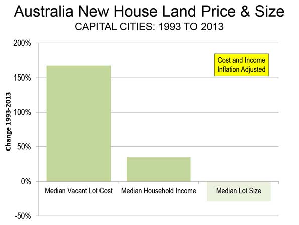
    For seven decades urban planners have been seeking to force higher urban population densities through urban containment policies. The object is to combat "urban sprawl," which is the theological (or ideological) term applied to the organic phenomenon of urban expansion. This has come at considerable cost, as house prices have materially increased relative to incomes, which is to be expected from urban containment strategies that ration land (and thus raise its price, all things being equal).

    Smart Growth America is out with its second report that rates urban sprawl, with the highest scores indicating the least sprawl and the lowest scores indicating the most (Measuring Sprawl 2014).

    Metropolitan Areas and Metropolitan Divisions

    For the second time in a decade Smart Growth America has assigned a "sprawl" rating to what it calls metropolitan areas. I say "what it calls," because, as a decade ago, the new report classifies "metropolitan divisions" as metropolitan areas (Note 1). Metropolitan divisions are parts of metropolitan areas. This is not to suggest that a metropolitan division cannot have a sprawl index, but metropolitan divisions have no place in a ranking of metropolitan areas. Worse, metropolitan areas with metropolitan divisions were not rated (New York, Los Angeles, Chicago, Dallas-Fort Worth, Philadelphia, Washington, Miami, San Francisco, Detroit, and Seattle).

    This year’s highest rating among 50 major metropolitan areas (over 1,000,000 population) goes to part of the New York metropolitan area (the New York-White Plains-Wayne metropolitan division) at 203.36. The lowest rating (most sprawling) is in Atlanta, at 40.99. This contrasts with 2000, when the highest rating was in part of the New York metropolitan area (the New York PMSA), at 177.8, compared to the lowest, in the Riverside-San Bernardino PMSA portion of the since redefined Los Angeles metropolitan area, at 14.2. Boston is excluded due to insufficient data (Note 2)

    Rating Sprawl

    The sprawl ratings are interesting, though obviously I would have done them differently.

    Overall urban population density would seem to be a more reliable indicator (called urbanized areas in the United States, built-up urban areas in the United Kingdom, population centres in Canada, and urban areas just about everywhere else). For example, the Los Angeles metropolitan area (combining its two component metropolitan divisions), has an index indicating greater sprawl than Springfield, Illinois. Yet, the Los Angeles urban area population density is about four times that of Springfield (6,999 residents per square mile, compared to 1747 per square mile, approximately the same as bottom ranking Atlanta). The implication is that if Los Angeles were to replicate the individual ratings that make up its index, and covered (sprawled) over four times as much territory, it would be less sprawling than today.

    This case simply illustrates the fact that sprawl has never been well defined. Indeed, the world’s most dense major urban area, Dhaka (Bangladesh), with more than 15 times the urban density of Los Angeles and 65 times the urban density of Springfield, has been referred to in the planning literature as sprawling.

    Housing Affordability

    The principal problem with the report lies with its assertions regarding housing affordability. Measuring Sprawl 2014 notes that less sprawling areas have higher housing costs than more sprawling areas (Note 3). However, it concludes that the lower costs of transportation offset much more all of the difference. This conclusion arises from reliance the US Department of Housing and Urban Development (HUD) and US Department of Transportation (DOT) Location Affordability Index, which bases housing affordability for home owners on median current expenditures, not the current cost of buying the median priced home. Nearly two thirds of the nation’s households are home owners, and most aspire to be.

    HUD-DOT describes its purpose as follows:

    "The goal of the Location Affordability Portal is to provide the public with reliable, user-friendly data and resources on combined housing and transportation costs to help consumers, policymakers, and developers make more informed decisions about where to live, work, and invest." 

    Yet, a consumer relying on the Location Affordability Index could be seriously misled. The HUD-DOT index (Note 4) does not begin to tell the story to people seeking to purchase homes. The costs are simply out of pocket housing costs, regardless of whether the mortgage has been paid off and regardless of when the house was bought (urban containment markets have seen especially strong house price increases).An index including people who have no mortgage and people who have lower mortgage payments as a result of having purchased years ago cannot give reliable information to consumers in the market today.

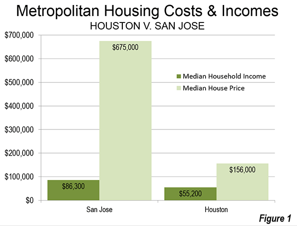
    A household relying on this source of information would be greatly misled. For example, comparing Houston with San Jose, according to HUD-DOT, owned housing and transportation consume virtually the same share of the median household income in each of the two metropolitan areas. In Houston, 52.5 percent of income is required for housing and transportation, while the number is marginally higher than San Jose (52.9 percent).

    But the HUD-DOT numbers reflect nothing like the actual costs of housing in San Jose relative to Houston. The median price house in Houston was approximately $155,000, 2.8 times the median household income of $55,200 (this measure is called the median multiple) during the 2006-10 period used in calculating the HUD-DOT index. In San Jose, the median house price was approximately $675,000, 7.8 times the median household income of $86,300 (Figure 1).

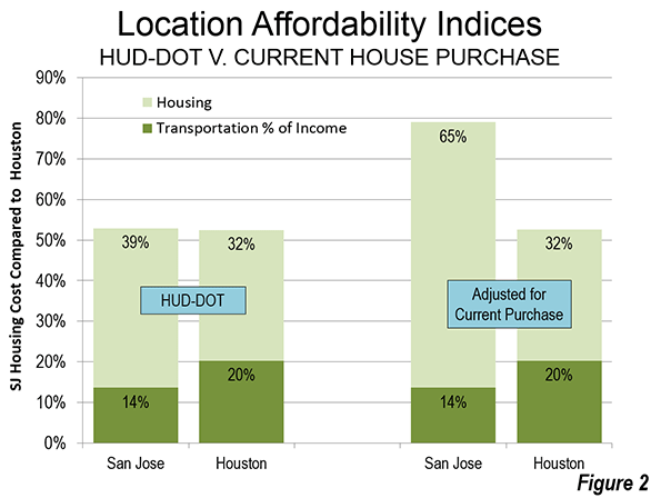
    If the Location Affordability Index reflected the real cost for a prospective home owner (HUD-DOT costs including a market rate mortgage for the house), a considerable difference would emerge between San Jose and Houston. The combined San Jose Location Affordability Index for home owners would rise to 85 percent of median household income, a full 60 percent above the Houston figure, rather than the minimal difference of less than one percent indicated by HUD-DOE (Figure 2).

    Under-Estimating the Cost of Urban Containment

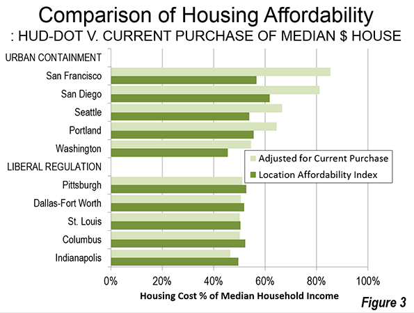
    There is a substantial difference between the HUD–DOT housing and transportation cost and the actual that would be paid by prospective buyers. Five selected urban containment markets indicate a substantially higher actual housing cost than reflected in the HUD–DOT figures. On the other hand, in the selected liberally regulated markets (or traditionally regulated markets), the HUD–DOE figure is much closer to the current cost of home ownership (Figure 3). This is a reflection of the greater stability (less volatility) of house prices in liberally regulated markets. Overall, based on data in the 50 major metropolitan areas, owned housing costs relative to incomes rise approximately 6 percent for each 10 percent increase in the sprawl index – that is, less sprawl is associated with higher house prices relative to incomes (Note 6).

    The increasing impacts of urban containment’s housing cost increases have been limited principally to households who have made recent purchases. The effect will become even more substantial in the years to come as the turnover of the more expensive housing stock continues.

    Granted, the 2006 to 2010 housing data includes part of the housing bubble and its higher house prices. However, house prices relative to incomes have returned to levels at or above that recorded during the period covered by Measuring Sprawl 2014 in "urban containment" markets, such as San Francisco, San Jose, Los Angeles, San Diego, Seattle, Portland, and Washington.

    Economic Mobility and Human Behavior

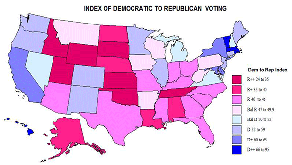
    Another assertion requires attention: economic mobility is greater in less sprawling metropolitan areas. The basis is research by Raj Chetty and Nathaniel Hendren of Harvard University and Patrick Kline and Emmanuel Saez of the University of California, Berkeley. However, the realities of domestic migration suggest caution with respect to the upward mobility conclusions, as is indicated in Distortions and Reality About Income Mobilityand in commentary by Columbia University urban planner David King.

    Virtually all urban history shows city growth to have occurred as people have moved to areas offering greater opportunity. Jobs, not fountains, theatres and art districts, drive nearly all the growth of cities. This means that there should be a strong relationship between the cities net domestic migration and the economic mobility conclusions of the research. The strongest examples show the opposite relationship.

    Domestic migration is strongly away from some metropolitan areas identified in the research as having the greatest upward income mobility also had substantial net domestic migration losses. For example, despite claims of high economic mobility New York, Los Angeles and the San Francisco Bay area, each lost approximately 10 percent of their population to net domestic migration in the 2000s. On the other hand, some metropolitan areas scoring the lowest in upward economic mobility drew substantial net domestic migration gains. For example, low economic mobility Charlotte and Atlanta gained 17 percent and 10 percent due to net domestic migration in the 2000s. Thus, the results of the economic research appear to be inconsistent with expected human behavior (Note 7).

    Sprawl: An Inappropriate Priority

    The new sprawl report is just another indication that urban planning policy has been elevated to a more prominent place than appropriate among domestic policy priorities. The usual justification for urban containment is a claimed sustainability imperative for its densification and anti-mobility policies. Yet, these policies are hugely expensive and thus ineffective at reducing greenhouse gas emissions, and thus have the potential to unduly retard economic growth (read "the standard of living and job creation"). Far more cost-effective alternatives are available, which principally rely on technology.

    There is a need to reverse this distortion of priorities. Little, if anything is more fundamental than improving the standard of living and reducing poverty (see Toward More Prosperous Cities). Housing is the largest element of household budgets and policies of that raise its relative costs necessarily reduce discretionary incomes (income left over after paying taxes and paying for basic necessities). There is no legitimate place in the public policy panoply for strategies that reduce discretionary incomes.

    London School of Economics Professor Paul Cheshire may have said it best, when he noted that urban containment policy is irreconcilable with housing affordability.

    ———

    Note 1: The previous Smart Growth America report used primarily metropolitan statistical areas (PMSAs), which have been replaced by metropolitan divisions. The primary metropolitan statistical areas were also subsets of metropolitan areas (labor market areas). This is problem is best illustrated by the fact that the Jersey City PMSA, composed only of Hudson County, NJ, is approximately one mile across the Hudson River from Manhattan in New York. Manhattan is the world’s second largest central business district and frequent transit service connects the two. Obviously, Jersey City is a part of the New York metropolitan area (labor market area), not a separate labor market.

    Note 2: Because of incomplete data, Boston is not given a sprawl rating in Measuring Sprawl 2014. A different rating system in the previous edition resulted in a Boston rating among the least sprawling. Yet, the Boston metropolitan area is characterized by low density development. Outside a 10 mile radius from downtown, the population density within the urban area is slightly lower than that of Atlanta (same square miles of land area used).

    Note 3: Higher house prices relative to household incomes are more associated with policies to control urban sprawl (such as urban growth boundaries and other land rationing devices), than with the extent of sprawl. More compact (less sprawling) urban areas do not necessarily have materially higher house prices. For example, in 1970, the Los Angeles urban area was one of the most dense in the United States, yet it was within the historical affordability range (a median multiple of less than 3.0). The emergence of Los Angeles as the nation’s most dense urban area in the succeeding decades (and 30 percent increase in density) is largely the result of a change in urban area criteria. Through 1990, the building blocks of urban areas were municipalities, which meant that many square miles of San Gabriel Mountains wilderness were included, because it was in the city of Los Angeles. Starting in 2000, the building blocks or urban areas became census blocks, which are far smaller and thus exclude the large swaths of rural territory that were included before in some urban areas.

    Note 4: The transport costs from the Location Affordability Index are accepted for the purposes of this article.

    Note 5: The current purchase housing cost is based on the average price to income multiple over the period of 2006 to 2010, relative to the median household income (calculated from quarterly data from the Joint Center for Housing Studies of Harvard University, State of the Nation’s Housing 2011). It is assumed that the buyer would finance 90 percent of the house cost at the average 30 year fixed mortgage rate with points over the period. The 10 percent down payment is allocated annually in equal amounts over the 360 months (30 years). The final annual cost estimate is calculated by adding the monthly mortgage payment and down payment allocation to the median monthly housing cost in each metropolitan area for households without a mortgage.

    HUD-DOT uses the "selected monthly owner cost" from the American Community Survey (ACS) for its cost of home ownership. According to ACS, “Selected monthly owner costs are calculated from the sum of payment for mortgages, real estate taxes, various insurances, utilities, fuels, mobile home costs, and condominium fees."

    Note 6: This is based on a two-variable regression estimation (log-log) with the sprawl index as the independent variable and the substituted housing share of income as the dependent variable for the 50 largest metropolitan areas (excluding Boston), It is posited that most of the variation in housing costs is accounted for by variation in land costs. Other significant factors, such as construction costs and financing costs in this sample vary considerably less. A sprawl index for each metropolitan areas represented by metropolitan divisions (not provided in the sprawl report) is estimated by population weighting.

    Note 7: Another difficulty with that research is that it measured geographic economic mobility at age 30, well before people reach their peak earning level. This is likely to produce less than reliable results, since those who achieve the highest incomes as well as the most educated such as medical doctors and people with advanced degrees) are likely to have larger income increases after age 30 than other workers.

    Wendell Cox is principal of Demographia, an international public policy and demographics firm. He is co-author of the “Demographia International Housing Affordability Survey” and author of “Demographia World Urban Areas” and “War on the Dream: How Anti-Sprawl Policy Threatens the Quality of Life.” He was appointed to three terms on the Los Angeles County Transportation Commission, where he served with the leading city and county leadership as the only non-elected member. He was appointed to the Amtrak Reform Council to fill the unexpired term of Governor Christine Todd Whitman and has served as a visiting professor at the Conservatoire National des Arts et Metiers, a national university in Paris.

    Suburban neighborhood photo by Bigstock.

  • Texas & Oklahoma Dominate Metropolitan Economic Growth

    Texas metropolitan areas continue to dominate economic growth, according to the latest Metro Monitor, produced by the Brookings Institution. The four top metropolitan areas in overall economic growth through the recession and "recovery" (our parentheses) have been:

    1. Austin
    2. Houston
    3. Dallas-Fort Worth
    4. San Antonio

    Oklahoma City took the 5th position. Oklahoma City, located 200 miles north of Dallas-Fort Worth may be experiencing some "overspill" economic growth from nearby Texas.

  • Concentrated Wealth or Democracy, but Not Both

    In many uncomfortable ways, American politics now resemble those that arose late in the Roman Republic. As wealth and land ownership concentrated in few hands, a state built on the discipline of soldiers who tended their own farms became ever more dominated by fractious oligarchs. As property consolidated into huge slave-owning estates, more citizens became landless and ever more dependent on the patronage of the rich generals and landowners who increasingly seized control of politics.

    In much the same way, as the wealth has concentrated in America, so, too, has the power exercised by those with money. The wealthy have always played an outsized role in our politics, but today, emboldened by Supreme Court rulings easing controls on contributions, oligarchs are dominating the electoral map in ways that have not been seen at least since the abuses of the Nixon years.

    Perhaps the most notable, or infamous, example is the Koch brothers, David and Charles, billionaire industrialists whose role in conservative politics has made them the ultimate “bogeymen” for crusading liberal journalists concerned with the growing power of the ultrarich on our political system. Campaigning against the Kochs has become standard issue for Democrats such as Senate Majority Leader Harry Reid.

    What makes the Koch brothers such great targets is that they come from an industry – energy – that itself is held in the lowest esteem by the progressive activist community and its media allies. Although they tend to be libertarian in their social views, the Kochs are notably, and not surprisingly, skeptical about climate change policies that might impact their vast oil and gas holdings as well as their industrial companies, which, in the words of former New York Times columnist Frank Rich, “spew” such unhappy products as Lycra and Dixie cups. The Kochs’ ties to the Tea Party have led reliably liberal commentators to suggest that the moguls have played the supposedly grass-roots Tea Party for “suckers.”

    As they rail against the Kochs, few progressives note that the balance of oligarchic politics are increasingly shifting toward the Democratic Party. This, of course, includes the predictable Hollywood figures, such as Dreamworks’ Jeffrey Katzenberg and a large section of Wall Street, notably financier George Soros, long a major source of funding for President Obama.

    These well-heeled progressives have had little to fear from an administration that, despite its occasional populist outbursts, has adopted an economic policy that has exacerbated an already yawning gap in income growth between the wealthy and everyone else. Indeed, Obama, for all his populist rhetoric, retained close ties to firms like Goldman Sachs, staffing his administration with people from, and associated with, that most-detested of Wall Street firms. Indeed the ultrarich so backed the ostensibly left-wing president that, at his first inaugural, notes sympathetic chronicler David Callahan, the biggest problem for donors was finding sufficient parking space for their private jets.

    An examination of campaign contributions shows that the vast majority of America’s wealthiest households may already tilt in this direction. Among the .01 percent who increasingly dominate political giving, three of the largest contributions, besides the conservative Club for Growth, backed by Republican oligarchs, went to groups such as Emily’s List, Act Blue and Moveon.org. Liberal groups accounted for eight of the top 10 ideological causes of the ultra-rich; seven of the 10 congressional candidates most dependent on their money were Democrats.

    This ideological shift among the rich, particularly the new rich, in what author Chrystia Freeland has dubbed an “age of elites,” is critical to understanding contemporary political conflict. There have always been, of course, affluent individuals who backed liberal or Democratic causes, out of a mixture of philosophy and self-interest but, for the most part, the wealthy backed Republicans. This has begun to change.

    Perhaps most ominous for the Right, the biggest growth in oligarchic politics has been from the very group – the so-called “high tech community” – that has flourished under the current easy-money regime. Once primarily middle-of-the-road Republican, the tech oligarchs have moved “left” in their politics, particularly on social and environmental issues. Many also have profited, or attempt to, through “green” energy investments. The leading tech companies, mostly based in the Silicon Valley, routinely send over four-fifths of their contributions to Democratic candidates.

    For the political parties, which are losing influence with every election, the rise of the oligarchs in politics represents a mixed blessing. To be sure, the tens of millions poured into the coffers of party candidates is welcomed, but at the same time, the oligarchs have become so powerful that they have altered, likely for a long time, the nominating and electing process.

    Republicans, for example, must deal with the likes of casino billionaire Sheldon Adelson, whose millions kept the quixotic, and seemingly pointless, Newt Gingrich campaign alive in the most-recent presidential primary campaign. The Koch brothers and others have also supported the supposedly grass-roots Tea Party, whose opposition to the Republican establishment has roiled GOP politics since 2010 and ended up with the nomination of some weak candidates.

    This year, it may be the Democrats’ chance to lament the rise of the oligarchs. At a time when economic growth and inequality are primary issues to most Americans, the presence of oligarchs all but guarantees that other issues – notably, environmental issues or social concerns like gay marriage – dominate the party’s fundraising. After all, it’s hard to imagine a party increasingly dependent on the wealthy seriously advocating, for example, for the equalization of capital gains and regular income taxes.

    Nobody better epitomizes the rise of economic royalist politics in the Democratic Party than San Francisco-based hedge-fund billionaire and green-energy investor Tom Steyer. Steyer has pledged to work against any Democrat who dares express the slightest skepticism about the need to diminish use of fossil fuels, no matter the economic cost. This could prove particularly tough on Democrats from energy states, like Louisiana, Texas, the Dakotas, Colorado and Montana, who historically have supported the fossil fuel industry as a prime generator of high-wage employment, including thousands of unionized blue-collar jobs.

    With Steyer pledging some $100 million to his anti-oil campaign, centered on opposition to the Keystone XL pipleline, the party is running against the popular grain. According to a recent Washington Post poll, the project is favored among the public by a margin of roughly three to one.

    So, Democrats find themselves pressured to oppose something favored by a large majority, all for an issue – climate change – that barely rates as a priority among voters far more worried about their jobs and families than carbon emissions. Just as well-financed Tea Party extremists have led the Republicans to nominate some lamentable candidates, Steyer’s efforts could undermine Democratic prospects – at least outside the solid coastal precincts – by forcing party figures further toward the gentry version of the Left.

    Ultimately, the biggest issue revolves not around the politics of the oligarchs but their overall potential to dominate our entire political culture. As Supreme Court Justice Louis Brandeis suggested in the last century, “We can have democracy in this country, or we can have great wealth concentrated in the hands of a few, but we can’t have both.”

    The founders, too, understood this basic truth. James Madison embraced the ideal of dispersed property – “the possession of different degrees and kinds of property” – as necessary in a functioning republic. Thomas Jefferson, admitting that the “equal division of property” was “impractical,” believed “the consequences of this enormous inequality producing so much misery to the bulk of mankind” that “legislators cannot invent too many devices for subdividing property.”

    It’s time we started listening to Brandeis and the founders. Until we address this issue of concentrated economic power – be it in the hands of oil barons or tech types – our politics will continue to devolve like those of Rome in the late Republic, undermining the last vestiges of citizen-based politics. Whether or not it results in the rise of an actual Caesar, this could be a sad day for what is left of our old Republic.

    This story originally appeared at The Orange County Register.

    Joel Kotkin is executive editor of NewGeography.com and Distinguished Presidential Fellow in Urban Futures at Chapman University, and a member of the editorial board of the Orange County Register. He is author of The City: A Global History and The Next Hundred Million: America in 2050. His most recent study, The Rise of Postfamilialism, has been widely discussed and distributed internationally. He lives in Los Angeles, CA.

    Photo by Peoplesworld.