Tag: Indianapolis

  • Time to Dismantle the American Dream?

    For some time, theorists have been suggesting that it is time to redefine the American Dream of home ownership. Households, we are told, should live in smaller houses, in more crowded neighborhoods and more should rent. This thinking has been heightened by the mortgage crisis in some parts of the country, particularly in areas where prices rose most extravagantly in the past decade. And to be sure, many of the irrational attempts – many of them government sponsored – to expand ownership to those not financially prepared to bear the costs need to curbed.

    But now the anti-homeowner interests have expanded beyond reigning in dodgy practices and expanded into an argument essentially against the very idea of widespread dispersion of property ownership. Social theorist Richard Florida recently took on this argument, in a Wall Street Journal article entitled “Home Ownership is Overvalued.”

    In particular, he notes that:

    The cities and regions with the lowest levels of homeownership—in the range of 55% to 60% like L.A., N.Y., San Francisco and Boulder—had healthier economies and higher incomes. They also had more highly skilled and professional work forces, more high-tech industry, and according to Gallup surveys, higher levels of happiness and well-being. (Note)

    Florida expresses concern that today’s economy requires a more mobile work force and is worried that people may be unable to sell their houses to move to where jobs can be found. Those who would reduce home ownership to ensure mobility need lose little sleep.

    The Relationship Between Household Incomes and House Prices

    It is true, as Florida indicates, that house prices are generally higher where household incomes are higher. But, all things being equal, there are limits to that relationship, as a comparison of median house prices to median house prices (the Median Multiple) indicates. From 1950 to 1970 the Median Multiple averaged three times median household incomes in the nation’s largest metropolitan areas. In the 1950, 1960 and 1970 censuses, the most unaffordable major metropolitan areas reached no higher than a multiple of 3.6 (Figure).

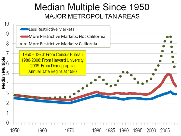
    This changed, however, in some areas after 1970, spurred by higher Median Multiples occuring in California.

    William Fischel of Dartmouth has shown how the implementation of land use controls in California metropolitan areas coincided with the rise of house prices beyond historic national levels. The more restrictive land use regulations rationed land for development, placed substantial fees on new housing, lengthened the time required for project approval and made the approval process more expensive. At the same time, smaller developers and house builders were forced out of the market. All of these factors (generally associated with “smart growth”) propelled housing costs higher in California and in the areas that subsequently adopted more restrictive regulations (see summary of economic research).

    During the bubble years, house prices rose far more strongly in the more highly regulated metropolitan areas than in those with more traditional land use regulation. Ironically many of the more regulated regions experienced both slower job and income growth compared to more liberally regulated areas, notably in the Midwest, the southeast, and Texas.

    Home Ownership and Metropolitan Economies

    The major metropolitan areas Florida uses to demonstrate a relationship between higher house prices and “healthier economies” are, in fact, reflective of the opposite. Between August 2001 and August 2008 (chosen as the last month before 911 and the last month before the Lehman Brothers collapse), Bureau of Labor Statistics data indicates that in the New York and Los Angeles metropolitan areas, the net job creation rate trailed the national average by one percent. The San Francisco area did even worse, trailing the national net job creation rate by 6 percent, and losing jobs faster than Rust Belt Pittsburgh, St. Louis, and Milwaukee.

    Further, pre-housing bubble Bureau of Economic Analysis data from the 1990s suggests little or no relationship between stronger economies and housing affordability as measured by net job creation. The bottom 10 out of the 50 largest metropolitan areas had slightly less than average home ownership (this bottom 10 included “healthy” New York and Los Angeles). The highest growth 10 had slightly above average home ownership (measured by net job creation). Incidentally, “healthy” San Francisco also experienced below average net job creation, ranking in the fourth 10.

    Moreover, housing affordability varied little across the categories of economic growth (Table).

    Net Job Creation, Housing Affordability & Home Ownership
    Pre-Housing Bubble Decade: Top 50 Metropolitan Areas (2000)
    Net Job Creation: 1990-2000 Housing Affordability: Median Multiple (2000) Home Ownership: Rate 2000
    Lowest Growth 10  7.4%                                2.8 62%
    Lower Growth 10 14.9%                                3.1 63%
    Middle 10 22.8%                                3.2 64%
    Higher Growth 10 30.9%                                2.6 61%
    Highest Growth 10 46.9%                                2.9 63%
    Average 24.7%                                2.9 62%
    Calculated from Bureau of the Census, Bureau of Economic Analysis and Harvard Joint Housing Center data.
    Metropolitan areas as defined in 2003
    Home ownership from urbanized areas within the metropolitan areas.

    Home Ownership and Happiness

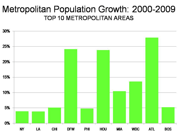
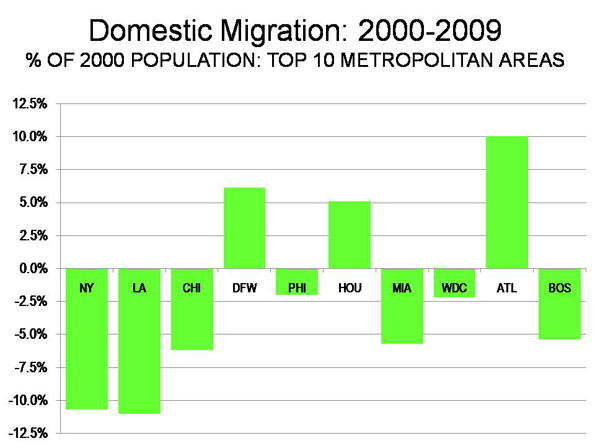
    If Gallup Polls on happiness were reliable, it would be expected that the metropolitan areas with happier people would be attracting people from elsewhere. In fact, people are fleeing with a vengeance. During this decade alone, approximately one in every 10 residents have left for other areas.

    • The New York metropolitan area lost nearly 2,000,000 domestic migrants (people who moved out of the metropolitan area to other parts of the nation). This is nearly as many people as live in the city of Paris.
    • The Los Angeles metropolitan area has lost a net 1.35 million domestic migrants. This is more people than live in the city of Dallas.
    • The San Francisco metropolitan area lost 350,000 domestic migrants. Overall, the Bay Area (including San Jose) lost 650,000, more people than live in the cities of Portland or Seattle.

    Why have all of these happy people left these “healthy economies?” One reason may be that so many middle income people find home ownership unattainable is due to the house prices that rose so much during the bubble and still remain well above the historic Median Multiple. People have been moving away from the more costly metropolitan areas. Between 2000 and 2007:

    • 2.6 million net domestic migrants left the major metropolitan areas (over 1,000,000 population) with higher housing costs (Median Multiple over 4.0).
    • 1.1 net domestic migrants moved to the major metropolitan areas with lower house prices (Median Multiple of 4.0 or below).
    • 1.6 million domestic migrants moved to small metropolitan areas and non-metropolitan areas (where house prices are generally lower).

    An Immobile Society?

    Florida’s perceived immobility of metropolitan residents is curious. Home ownership was not a material barrier to moving when tens of millions of households moved from the Frost Belt to the Sun Belt in the last half of the 20th century. During the 2000s, as shown above, millions of people moved to more affordable areas, at least in part to afford their own homes.

    Under normal circumstances (which will return), virtually any well-kept house can be sold in a reasonable period of time. More than 750,000 realtors stand ready to assist in that regard.

    Of course, one of the enduring legacies of the bubble is that many households owe more on their houses than they are worth (“under water”). This situation, fully the result of “drunken sailor” lending policies, is most severe in the overly regulated housing markets in which prices were driven up the most. Federal Reserve Bank of New York research indicates that the extent of home owners “under water” is far greater in the metropolitan markets that are more highly restricted (such as San Diego and Miami) and is generally modest where there is more traditional regulation, such as Charlotte and Dallas (the exception is Detroit, caught up in a virtual local recession, and where housing prices never rose above historic norms, even in the height of the housing bubble). Doubtless many of these home owners will find it difficult to move to other areas and buy homes, especially where excessive land use regulations drove prices to astronomical levels.

    Restoring the Dream

    There is no need to convince people that they should settle for less in the future, or that the American Dream should be redefined downward. Housing affordability has remained generally within historic norms in places that still welcome growth and foster aspiration, like Atlanta, Dallas-Fort Worth, Houston, Indianapolis, Kansas City, Columbus and elsewhere for the last 60 years, including every year of the housing bubble. Rather than taking away the dream, it would be more appropriate to roll back the regulations that are diluting the purchasing power and which promise a less livable and less affluent future for altogether too many households.

    Note. Among these examples, New York is the largest metropolitan area in the nation. Los Angeles ranks number 2 and San Francisco ranks number 13. The inclusion of Boulder, ranked 151st in 2009 seems a bit curious, not only because of its small size, but also because its advantage of being home to the main campus of the University of Colorado. Smaller metropolitan areas that host their principal state university campuses (such as Boulder, Eugene, Madison or Champaign-Urbana) will generally do well economically.

    Photograph: New house currently priced at $138,990 in suburban Indianapolis (4 bedroom, 2,760 square feet). From http://www.newhomesource.com/homedetail/market-112/planid-823343

    Wendell Cox is a Visiting Professor, Conservatoire National des Arts et Metiers, Paris. He was born in Los Angeles and was appointed to three terms on the Los Angeles County Transportation Commission by Mayor Tom Bradley. He is the author of “War on the Dream: How Anti-Sprawl Policy Threatens the Quality of Life.

  • The New Look of the American Suburb

    If you want an easy demonstration of the unsustainability of the classic American suburb, just take a drive around the inner ring suburbs of almost any city, starting with the ones that have a classic branching, winding streets, not traditional grids or those that grew up along transit lines. It is easy to find untold miles of decay, of “dead malls”, “grayboxes”, and subdivisions that have seen better days. If most of today’s new suburbs think they’ll fare any better, they are going to be in for a rude shock in 30 years or so.

    Some have argued that what we need are “suburban retrofits,” where older areas are redeveloped along new urbanist lines. While this is certainly an attractive option in some places, particularly in town center areas, the sheer quantity of decaying older suburbs means this isn’t a viable option across the board at the moment. Retrofits are hard to pull off and expensive to boot. There simply isn’t enough planner/political bandwidth or TIF dollars to make it happen on a wholesale basis. So we have to find some method to renew most of these areas in place.

    Enter immigrants. In older cities, immigrants were historically crammed into near downtown ghettos like the various “Chinatowns” and the like we see. Today, in cities that have them, those districts might still have a cultural role, but they are no longer the demographic core of their communities. Also, for cities without longstanding histories of immigration, these ghettos never developed. Instead, today immigrants disperse throughout metro areas. You find them everywhere from inner city neighborhoods to the most posh suburbs. One of the places along that spectrum you can find them are these inner ring suburbs.

    I want to share some pictures of immigrant driven revitalization of inner ring suburbs through some facts and photos from Indianapolis. But I think you’d find similar things in many cities across the nation.

    Indianapolis was traditionally one of America’s least diverse cities, featuring only the classic black-white split. But it has seen a large influx of immigrants in the last decade. Its metro foreign born population is only 5.19%, which is small, but the Indianapolis Star reported last year that this represented a 70% population increase since 2000. Unlike some towns which have seen immigration driven almost entirely from Mexico, Indianapolis has seen a very diverse set of immigrants, that come from all over the globe, including 26,000 Asians and 10,500 Africans. The Indian population has doubled to 6,000, the Pakistani and Nigerian populations have tripled to 1,000 each. There are 5,600 Chinese and 1,500 Burmese. These aren’t huge numbers today, but given the network effects of international immigration and the lead time to build a large community (remember the example of the large community from Tala, Mexico, which has its roots in the 1970’s), this represents a potential future tsunami of immigration, provided the economy stays strong, the local climate welcoming, and a bit of pro-active marketing takes place. Again, I’m sure we’d see similar diversity of immigrants in other cities, ranging from Detroit’s Arab community to Bosnians in St. Louis to Somalis in Columbus, Ohio.

    The most diverse area in Indianapolis is Pike Township on the northwest side. Though technically part of the city today, it is originally an inner ring suburban area. Its schools have children from 63 different countries speaking 74 different languages. The Lafayette Square area on the southeast boundary of Pike Township is a classic struggling inner ring commercial zone, complete with a dying mall.

    Yet the presence of all of those immigrants has led to a spontaneous renewal of parts of this struggling area in the form of businesses catering to local ethnic populations.

    One of them is a 62,000 square feet international supermarket called Saraga:


    Saraga is run by Korean brothers Jong Sung and Bong Jae Sung and features hundreds of spices and 40,000 products from around the world, ranging from house made kimchi to a halal meat department. Lest I stir up too much suspicion I didn’t take many photos inside the store, but wanted to share one shot of some of the contents from a Middle Eastern aisle:


    The owners are planning to open a second location on the South Side. They are facing a lot of competition from an array of new specialty markets in their current location, and also want to be positioned closer to the burgeoning immigrant community on the South Side and south suburbs. Not long ago the South Side of Indianapolis was stereotyped as the “redneck” side of town, but as American Dirt chronicled, this has changed a lot. While not part of the favored quarter, the South Side has increasing diversity both ethnically and in terms of incomes. Notably the South Side has become epicenter of the Indianapolis Sikh community.


    Saraga should be careful. There are already two Indian groceries and a Mexican grocery in Greenwood. Here is part of the competition in Lafayette Square:


    This, and many of the other establishments, might not look like much. But imagine what it would look like if they weren’t there.

    Here’s one of my favorite signs from a nearby strip center, showing the diversity of establishments rubbing elbows:


    The facade of Cairo Cafe shows a typical Indianapolis pattern, where an ethnic restaurant does double duty as a small scale specialty grocery.


    It’s the same thing at the Vietnamese restaurant Saigon and Guatelinda. Saigon is beloved of hipsters, but I’ve got to confess I don’t think it is very good.


    Another nearby strip mall always blows my mind for the diversity of restaurants and stores it contains. You might need to enlarge this one to see, but it’s a Peruvian restaurant next to a Mexican restaurant next to an Ethiopian restaurant:


    A pastry shop next to another oriental market:


    Some type of Latino shop:


    A Cuban sandwich shop:


    Hopefully this gives you a flavor for how immigrants can be a force of renewal for older, struggling suburban area. I’ll admit I focused on food establishments, since that’s what’s most interesting to me, but there are plenty of others. This also shows the increasingly multi-cultural face of America, even in an interior city in the middle of Midwest corn country. If I were a city with lots of these struggling areas – and let’s face it, that’s most cities – I’d sure want to get me a lot more immigrants pronto.

    In the interest of completeness, I should also note that the Lafayette Square area has also become home to large number of independent black-owned businesses. In addition to being Indy’s immigrant heart, Pike Township has also emerged as a key hub for the region’s black middle class. That will have to be the topic of a future post, alas.

    Aaron M. Renn is an independent writer on urban affairs based in the Midwest. His writings appear at The Urbanophile.

    This article is re-posted from The Urbanophile.

  • SPECIAL REPORT: Metropolitan Area Migration Mirrors Housing Affordability

    On schedule, the annual ritual occurred last week in which the Census Bureau releases population and migration estimates and the press announces that people are no longer moving to the Sun Belt. The coverage by The Wall Street Journal was typical of the media bias, with a headline “Sun Belt Loses its Shine.” In fact, the story is more complicated – and more revealing about future trends.

    Domestic Migration Tracks Housing Affordability: There have been changes in domestic migration (people moving from one part of the country to another) trends in the last few years, but the principal association is with housing affordability.

    Severe and Not-Severe Bubble Markets: Overall, the major metropolitan markets with severe housing bubbles (a Median Multiple rising to at least 4.5, see note) lost nearly 3.2 million domestic migrants (all of these markets have restrictive land use regulation, such as smart growth or growth management) from 2000 to 2009. However, not all markets with severe housing bubbles lost domestic migrants. “Safety valve” bubble markets drew migration from the extreme bubble markets of coastal California, Miami and the Northeast. These “safety valve” markets (including Phoenix, Las Vegas, Portland, Seattle, Riverside-San Bernardino, Orlando, Tucson and Tampa-St. Petersburg), gained a net 2.2 million from 2000 to 2009, while the other bubble markets lost 5.3 million domestic migrants from 2000 to 2009 (See Table below, metropolitan area details in Demographia US Metropolitan Areas Table 8). At the same time, the markets that did not experience a severe housing bubble (those in which the Median Multiple did not reach 4.5) gained a net 1.5 million domestic migrants.

    The burst of the housing bubble explains the changes in domestic migration trends. Housing affordability has improved markedly in the extreme bubble markets, so that there was less incentive to move. Then there was the housing bust-induced Great Recession, which also slowed migration since people had more trouble selling their homes or finding anew job. As a result, the migration to the “safety valve” markets and to the smaller markets dropped substantially.

    • During 2009, the “safety valve” markets gained only 51,000 net domestic migrants, one-fifth of the annual average from 2000 to 2008.
    • At the same time, the other severe housing bubble markets lost 236,000 domestic migrants in 2009, compared to the average loss of 638,000 from 2000 to 2008.
    • Areas outside the major metropolitan areas also experienced a significant drop in domestic migration, dropping from an annual average of 203,000 between 2000 and 2008 to 23,000 in 2009.
    • The major metropolitan markets that did not experience a severe housing bubble gained 161,000 domestic migrants in 2009, little changed from the 169,000 average from 2000 to 2008. These markets are concentrated in the South and Midwest. Indianapolis, Kansas City, Nashville, Louisville and Columbus as well as the Texas metropolitan areas continued their positive migration trends.
    Domestic Migration by Severity of the Housing Bubble
    Metropolitan Areas over 1,000,000 Population
    2000-2008
    Metropolitan Areas 2000-2009 2009 2000-2008 Average
    Withouth Severe Housing Bubbles     1,509,870         160,514      168,670
    With Severe Housing Bubbles    (3,161,514)        (184,486)     (372,129)
       Not "Safety Valve" Markets    (5,347,211)        (235,838)     (638,922)
       "Safety Valve" Markets     2,185,697           51,352      266,793
    Outside Largest Metropolitan Areas     1,651,644           23,972      203,459
    Severe housing bubbles: Housing costs rose to a Median Multiple of 4.5 or more (50% above the historic norm of 3.0). 
    Median Multiple: Median House Price/Median Household Income
    "Safety Valve" refers to markets with severe housing bubbles that received substantial migration from more expensive markets (coastal California, Miami and the Northeast). These markets include Las Vegas, Phoenix, Riverside-San Bernardino, Sacramento, Portland, Seattle, Orlando, Tucson and Tampa-St. Petersburg.

    Moreover, the Census Bureau revised its previous domestic migration figures for 2000 to 2008 to add more than 110,000 from the markets without severe housing bubbles, while taking away more than 150,000 domestic migrants from the markets with severe housing bubbles. This adjustment alone rivals the 2009 domestic migration loss of 183,000 in these markets

    Population Growth: The Top 10 Metropolitan Areas: Sun Belt metropolitan areas continued to experience the greatest population growth. Between 2000 and 2009, the fastest growing metropolitan areas were Atlanta, Dallas-Fort Worth and Houston, In 2009, Washington, DC was added to the list (Details in Demographia US Metropolitan Areas, Table 2).

    New York: The New York metropolitan area remains the nation’s largest, now reaching a population of over 19 million. More than 700,000 new residents have been added since 2000. However, New York’s population growth has been the second slowest of the 10 largest metropolitan areas since 2000 (Figure 1). Moreover, New York’s net domestic out-migration has been huge. New York has lost 1,960,000 domestic migrants, which is more people than live in the boroughs of The Bronx and Richmond combined. Overall, 10.7% of the New York metropolitan area’s 2000 population left the metropolitan area between 2000 and 2009. More than 1,200,000 of this domestic migration was from the city of New York. Between 2008 and 2009, New York’s net domestic out-migration slowed from the minus 1.32% 2000-2008 annual rate to minus 0.58%., reflecting the smaller migration figures that have been typical of the Great Recession.

    Los Angeles: For decades, Los Angeles has been one of the world’s fastest growing metropolitan areas. Growth had ebbed somewhat by the 1990s, when Los Angeles added 1.1 million people. The California Department of Finance had projected that Los Angeles would add another 1.35 million people between 2000 and 2010. Yet, the Los Angeles growth rate fell drastically. From 2000 to 2009, Los Angeles added barely one-third the projected amount (476,000) and grew only 3.8%. Unbelievably, fast growing Los Angeles became the slowest growing metropolitan area among the 10 largest. In 2009, Los Angeles had 12.9 million people. Los Angeles lost 1.365 million domestic migrants, which is of 11.0% of its 2000 population, and the most severe outmigration among the top 10 metropolitan areas (Figure 2).

    Chicago: Chicago continues to be the nation’s third largest metropolitan area, at 9.6 million population, a position it has held since being displaced by Los Angeles in 1960. Chicago has experienced decades of slow growth and continues to grow less than the national average, at 5.1% between 2000 and 2009 (the national average was 8.8%). Yet, Chicago grew faster than both New York and Los Angeles. Chicago also lost a large number of domestic migrants (561,000), though at a much lower rate than New York and Chicago (6.2%). Even so, Chicago is growing fast enough that it could exceed 10 million population in little more than a decade, by the 2020 census.

    Dallas-Fort Worth: Dallas-Fort Worth has emerged as the nation’s fourth largest metropolitan area, at 6.4 million, having added 1,250,000 since 2000. In 2000, Dallas-Fort Worth ranked fifth, with 500,000 fewer people than Philadelphia, which it now leads by nearly 500,000. Dallas-Fort Worth added more population than any metropolitan area in the nation between 2008 and 2009 and has been the fastest growing of the 10 top metropolitan areas since 2006. As a result, Dallas-Fort Worth has replaced Atlanta as the high-income world’s fastest growing metropolitan area with more than 5,000,000 population. Dallas-Fort Worth added a net 317,000 domestic migrants between 2000 and 2009.

    Philadelphia: Philadelphia is the nation’s fifth largest metropolitan area, at just below 6,000,000 population. Like Chicago, Philadelphia has had decades of slow growth, yet has grown faster in this decade than both New York and Los Angeles (4.8%). Philadelphia has lost a net 115,000 domestic migrants since 2000, for a loss rate of 2.2%, well below that of New York, Los Angeles and Chicago.

    Houston: Houston ranks sixth, with 5.9 million people and is giving Dallas-Fort Worth a “run for its money.” Like Dallas-Fort Worth, Houston has added more than 1,000,000 people since 2000. Over the same period, Houston has passed Miami and Washington (DC) in population. Houston has added a net 244,000 domestic migrants since 2000, and added 50,000 in 2008-2009, the largest number in the country. Like Dallas-Fort Worth, Houston accelerated its annual domestic migration growth rate in 2008-2009. At the current growth rate, Houston seems likely to pass Philadelphia in population shortly after the 2010 census.

    Miami: Miami (stretching from Miami through Fort Lauderdale to West Palm Beach) is the seventh largest metropolitan area, with 5.6 million people. Miami has added more than 500,000 people, for a growth rate of 10.4%. However, Miami has suffered substantial domestic migration losses, at 287,000, a loss rate of, 5.7% relative to its 2000 population.

    Washington (DC): Washington recaptured 8th place, moving ahead of Atlanta, which had temporarily replaced it. Washington’s population is 5.5 million and added 655,000 between 2000 and 2009, for a growth rate of 13.6%. However, Washington lost a net 110,000 domestic migrants, 2.2% of its 2000 population. That trend was reversed in 2008-2009, when a net 18,000 domestic migrants moved to Washington, perhaps reflecting the increased concentration of economic power in the nation’s capital.

    Atlanta: Atlanta is the real surprise this year. For more than 30 years, Atlanta has had strong growth, however, this year it slowed. Atlanta is the 9th largest metropolitan area in the nation, at 5.5 million. Since 2000, Atlanta has added 1.2 million people, though added only 90,000 last year. Atlanta has added a net 429,000 domestic migrants since 2000, though the rate slowed to only 17,000 in 2008-2009.

    Boston: Boston is the nation’s 10th largest metropolitan area, with 4.6 million people. During the 2000s, Boston has added nearly 200,000, growing by 4.2%. Yet, Boston has also experienced a net domestic migration loss of 236,000, or 5.4% of its 2000 population. In 2008-2009, Boston, like Washington, reversed its domestic migration losses, adding 7,000.

    Trends by Size of Metropolitan Area: As throughout the decade, the slowest growing areas of the nation have been metropolitan areas over 10,000,000 population (New York and Los Angeles), which grew 3.9% and non-metropolitan areas, which grew 2.6% during the decade Metropolitan areas that had between 2.5 and 5.0 million population in 2000 boasted the biggest jump (these include fast growing Houston and Atlanta, which are now more than 5 million), at 13.4% for the decade. All of the other size classifications grew between 8.9% and 11.3% over the decade (see Demographia US Metropolitan Areas, Table 1). Metropolitan areas that began the decade with between 5,000,000 and 10,000,000 population gained 10.0%. Those with 250,000 to 500,000 grew 10.4%, those with 500,000 to 1,000,000 grew 10.2% and the smallest metropolitan areas, those from 50,000 to 250,000 grew 8.9%

    Metropolitan areas over 1,000,000 population lost 2.19 million domestic migrants during the decade, but smaller metropolitan areas added 2.24 million domestic migrants. Non-metropolitan areas lost 50,000 domestic migrants. In 2009, the smaller metropolitan areas gained 125,000 domestic migrants, while the larger metropolitan areas lost 30,000. Non-metropolitan areas lost more than 90,000 domestic migrants. As noted above, these smaller figures for 2009 reflect the more stable housing market and the extent to which the Great Recession has reduced geographic mobility (See Demographia US Metropolitan Areas, Tables 1 and 3).


    Note: The Median Multiple is the median house price divided by the median household income. The historic standard has been 3.0.

    Photograph: Dallas

    Wendell Cox is a Visiting Professor, Conservatoire National des Arts et Metiers, Paris. He was born in Los Angeles and was appointed to three terms on the Los Angeles County Transportation Commission by Mayor Tom Bradley. He is the author of “War on the Dream: How Anti-Sprawl Policy Threatens the Quality of Life.

  • Midwest Success Stories

    Most observers do not associate the Midwest with urban success, but quite the opposite in fact. But while there are plenty of places that are legitimately suffering, there are also plenty of success stories out there that don’t always get the mindshare or press they deserve.

    First on my list of Midwest success stories is Des Moines, Iowa. This is a smaller,, largely under the radar city, but it has emerged as one of the strongest performers anywhere in the United States. This city defines the term “easy living”, while still managing to be home to major industries like insurance. Being smaller has proven an asset here, as Des Moines has avoided many of the large scale boondoggles like pro sports stadiums cities sometimes engage in to try to prove they are “major league”.

    Instead of competing for bragging rights, Des Moines instead has grown its job base significantly during the “lost decade” of the 2000s. Between 2001 and 2009, it added over 25,000 jobs – a healthy 8.9% clip – and boasts a close to rock bottom (for these times) 6.5% unemployment rate. Des Moines metro grew its population at 15.5% between 2000 and 2008, nearly double the national average, belying the notion that no one wants to live in Iowa. Despite this growth, labor shortages remain a long term local concern. That’s called a nice problem to have.

    Indianapolis is another standout, with a profile closer to the Sun Belt than the Rust Belt. It grew its population at a rate 50% greater than the national average, and also had strong net in-migration,with almost 65,000 net people deciding to pack up and move to Indy. Its demographic and economic stats are very comparable to Portland, Oregon, the urban policy poster child. In fact, Indianapolis actually added more jobs than Portland – where job growth has been largely in the suburban periphery – last decade thanks to an aggressive pro-business attitude and local industry clusters like life sciences, motorsports, and internet marketing.

    Indianapolis may also be the least expensive major housing market in America, but it maintains a full range of urban amenities and is only three hours drive from Chicago for those things it lacks. This is one reason Business Week just named the large suburb of Fishers the best affordable suburb in the United States. Indy has also quietly established a position as an urban innovator, with unique to the nation projects like a downtown urban trail. It is also a leader in modern roundabouts, with suburban Carmel having 5% of all the modern roundabouts in the entire United States.

    Head east on I-70 and three hours later you’ll arrive in Columbus, Ohio, Indy’s “twin city”. Like Indianapolis, an artificially chosen state capital, Columbus is thriving in a struggling state. Like Indy, it also has strong population growth and net in-migration, and a below average unemployment rate. It’s home to powerhouse Ohio State University, which boasts the nation’s largest college campus, and stunning historic neighborhoods like German Village. Columbus is home to a thriving LGBT community, and the second largest gay pride parade in the Midwest after Chicago, one of the top ten in the country, attracting over 100,000 attendees.

    West along I-70 is Kansas City. Described as a “zone of sanity”, Kansas City avoided the housing boom and thus largely the bust, remaining another affordable and attractive place to live. It too has had strong population growth and net in-migration, along with below average unemployment. The city is the second largest rail hub in the United States after Chicago, but lacks that city’s legendary rail congestion. Unsurprisingly, rail carriers are investing heavily there. With rail connectivity to Mexican ports, and sitting along I-35, Kansas City is looking to be one of the winners of NAFTA. Plentiful fountains and miles of lush parkways make Kansas City a lovely city. It is also a cultural hub, with the respected Nelson-Aktins Museum at the high end and the thriving Crossroads Art District on the grass roots side.

    Madison, Wisconsin is one of the rare Midwest cities that actually gets national respect. Its location along a narrow isthmus creates a charming physical setting and compact urban core. Home to the University of Wisconsin, its progressive credentials are unimpeachable. But it is also an economic success story, with strong job growth of 6.6% from 2001-2009, along with impressive population growth. Part of this is the university’s powerhouse researchers, who attracted the likes of Google to open an office. The city is also the state capital. Despite being a smaller city, it boasts amenities worthy of America’s elite metropolises, including super-high end denim retailer Context Clothing and the luxurious Candinas Chocolatier.

    Despite its reputation for frigid weather and its geographically peripheral location, Minneapolis-St. Paul offers both economic strength and high quality of life. Its residents embrace the recreational opportunities provided by numerous nearby lakes, including several inside the Minneapolis city limits, as well as the winter. The region was early to the starchitect game, with Frank Gehry designing the metallic Weisman Art Center before the Bilbao Guggenheim. But it’s not all fun and games there. The region has an unemployment rate well below average and a GDP per capita well above it. It is home to numerous household name firms like Target, Best Buy, and 3M. And it is a center for the medical device industry.

    These six cities show that there’s a lot more to the Midwest than rusted steel mills, shuttered auto plants, and abandoned houses. It is also home to healthy cities and thriving suburban communities that are outpacing the nation demographically and economically. These places offer affordability and a high quality of life, but still manage to feature many more urban amenities and innovations than commonly assumed. These characteristics make them well-positioned to be among the urban winners in the 21st century.

    Aaron M. Renn is an independent writer on urban affairs based in the Midwest. His writings appear at The Urbanophile.

    Photo by Carl Van Rooy (vanrooy_13)

  • The 10 Percent Solution to Urban Growth

    What if we achieved the urbanist dream, with people deciding en masse to move back to the city? Well, that would create a big problem, since there would be no place to put them. Many cities hit their peak population in 1950, when the US total was 150 million. Today it is over 300 million, with virtually all the growth taking place in the suburbs.

    So where would these new urbanites reside? With the enormous losses in our urban housing stock, our cities lack the residences to hold even their 1950 population. A recent survey found that one third of all the lots in Detroit are now vacant, for example. And even if all the old housing was rebuilt, declines in household sizes, particularly in urban areas, has reduced the effective carrying capacity of the old urban fabric even at historic densities.

    But there’s an even bigger challenge to wholesale urbanization from future population growth. The Census Bureau estimates that the US will add nearly 100 million more new people by 2050. If you look at the few cities in the country that have large inhabited urban cores, they hold a relatively small percentage of the current population. New York City, Los Angeles, Chicago, Philadelphia, San Francisco, Boston, Seattle and Washington, DC combined barely hold 20 million people. Even if all these cities doubled in population by 2050, they would only be able to hold 20% of the net new growth expected over the next four decades.

    And achieving even that level of urban growth is simply not realistic. Most of the existing highly urbanized cities are already largely full of buildings. Even where land is available, zoning restricts what can be built there, and increasing densities is politically difficult. New York City has been the most aggressive on the growth front, rezoning 20% of the city under the Bloomberg administration, although many sections have actually been downzoned.

    But even this effort could accommodate a projected one million new residents by 2030. Chicago is going the other direction. When it introduced new zoning under the Daley administration, permitted densities were actually reduced in most cases, though Chicago remains perhaps the only truly urban city with large amount of vacant or underutilized land for redevelopment. Ed Glaeser calls for building skyscrapers in California, but San Francisco residents are imbued with a strong anti-development mindset and have long railed against the “Manhattanization” of their city.

    America could not be reshaped from a primarily suburban to a city-centric country without a massive shift in local political mind-sets. Rather than attempting that exercise in futility, urban advocates should adopt much more modest goals that, although limited, could be completely transformational for our cities.

    There’s been much made of the return to the city. Indeed, large tracts of the urban cores of many places have been utterly remade. But most of the cities where this has happened have been America’s largest tier one cities – New York, Chicago, Boston, etc. They have achieved the point of self-sustaining urban growth, and are well positioned to attract more residents, particularly the upscale and childless, young singles and students and recent immigrants.

    In contrast, smaller cities have seen a few hundred downtown condos and such, but not a real urban renaissance. There is still a lot of work to do in those places.

    The way to do this is to adopt the “10 percent solution”. That is, for most cities, they should develop a strategy that tries to capture somewhere between 5 and 15 percent of the net new growth in their metro areas. If a city can get more, great. But for any growing region, even 10 percent would create a dynamic of massive change in the urban core.

    Consider Indianapolis, a region with healthy regional growth that is above average but not among the nation’s leaders. The Indianapolis metro area is adding people at a rate of about 200,000 people per decade. Center Township, which is the urban core of the city, peaked in population in 1950 at 337,000 people. Today it is at 167,000, a decline of 50%, on par with America’s greatest urban collapses

    But what if the urban core managed to capture 10% of that new growth? That’s 20,000 new residents, very easy to physically accommodate within a decade. What would 20,000 new residents do to central Indianapolis? What would it do to the entire dynamic of the city? It could be completely transformational.

    Such a modest capture of new population would catapult central Indianapolis into one of the absolute top growth areas in the region. Only one suburb is on track to add that many or more people during the 2000s. Many other suburbs are considered prosperous and fast growing despite adding only a few thousand people. Even that limited influx creates a pattern of growth vs. stagnation and decline. That’s where urban Indianapolis needs to get.

    One of the great advantages of targeting 10% market share in new growth is that it frees the city to pursue a market segmentation strategy. It doesn’t have to try to convince vast numbers of suburbanites – the vast majority of whom are likely to stay in place – to make a radical lifestyle change. Rather, the core can market to specific segments that it is best positioned to attract, and put together the most compelling and differentiated product to attract them.

    One potential market is those who want an urban environment but can’t afford to live in one of the expensive tier one cities. They could market themselves to people who find themselves priced out of the biggest cities, but would settle in a smaller, but still vibrant urban environment.

    Can Indianapolis do it? As with many cities, there is already some evidence that it could. In the 2000s, decades of population decline came to an end in 2006, and Center Township started adding an estimated 400 people per year. The jury is still out on whether the estimates are confirmed by the census count and whether it can be sustained, but it still amounts to 4,000 people per decade, showing that the city is already starting to make progress.

    Cincinnati provides another example. It is a metro growing a bit less than the national average, but still adding people at a rate of about 150,000 per decade. The city of Cincinnati declined from a peak of 503,998 in 1950 to 333,336 today, a loss of 170,000 people. Again, if the city captured 100% of just regional growth, in little more than a decade it would be back to a record high population. That’s not realistic of course, but 10% of that total, or 15,000 people, would still make a tremendous impact on the city. Like Indianapolis, there’s already some sign of an inflection point, as the city population began growing again in the 2000s.

    Can this 10% solution really happen? The answer is a resounding Yes, because it is already happening in Atlanta. Its reputation as a sprawlburg overshadows the fact that it is experiencing one of America’s most impressive urban core booms. The city of Atlanta has added almost 120,000 new residents since 2000, an increase of 28%. This is a mere 10.5% of the metro area’s growth during that time – but it has totally changed the city. Atlanta lost over 100,000 people from its 1970 peak, but is now at an all time high.

    Viewed in this realistic light, there is huge reason for optimism about rebuilding the urban cores of even our Rust Belt cities. Frankly, with the required market share of growth to get there so low, there’s no excuse for not making it happen. If city leaders can’t figure out how to attract even 10% of the market, they deserve to lose. If they can do better, great. And once they’ve captured that 10% base, and restarted a growth pattern, they can figure out how to get more ambitious and expand market share.

    For regions with population decline, like Detroit and Cleveland, there’s a different and much more challenging dynamic. But for cities with even modest regional population growth, there’s all the opportunity in the world to attract new urban residents and completely change the game for their urban cores.

    Aaron M. Renn is an independent writer on urban affairs based in the Midwest. His writings appear at The Urbanophile.

    Photo: Carl Van Rooy (vanrooy_13)

  • “First” vs. “Worst”

    Taking on the Portland mystique is not easy – and likely I’ll find out again with my most recent piece: Picture-perfect Portland?

    But I’d also like to take a Midwest perspective that shows some surprising things. Let’s compare Portland to a similarly sized and less acclaimed Midwest city, Indianapolis. You can think of Portland as being in “first place” from a policy perspective by popular acclaim. It has an urban growth boundary, extensive transit, excellent urban density, a strong biking culture, a strong culture of civic engagement, the most microbreweries per capita, and on down the line. It is a place people want to live in so badly that they will move there with no job in hand and would be one of the cities that comes to mind among similar sized metros as a talent hub.

    If Portland is first, then you’d have to characterize Indianapolis as “worst”. Indianapolis is surrounded by expanding suburbia with very pro-sprawl policies on all four sides. It is one of the least dense cities in America. It has no rail transit and only the 99th largest bus system, along with one of the lowest transit market shares in the country. It is currently in the middle of a multi-billion program to widen about 60 miles of freeway. It just recently put in its very first bike lanes and scores near the bottom in green measures of sustainability. Its brand image also is hardly the best. You don’t hear too many people around the country going, “Man, I’ve gotta get me to Indianapolis.”

    But let’s look at how these cities compare on various quantitative measures of urban performance.


    Portland

    Indianapolis

    Population Growth (2000-2008)

    14.5%

    12.5%

    Domestic In-Migration (2000-2008)

    5.4%

    4.2%

    International In-Migration (2000-2008)

    3.7%

    1.4%

    Job Growth 2001-2009 (QCEW)

    10,300 (1.1%)

    17,100 (2.1%)

    Job Growth 2001-2009 (CES)

    23,800 (2.4%)

    31,000 (3.6%)

    Unemployment Rate (Nov 2009)

    10.8%

    8.2%

    Per Capita GMP (2008)

    47,811

    46,450

    Per Capital GMP Growth (2001-2008)

    22.4%

    1.7%

    Median Household Income (ACS 2008)

    $58,758

    $53,671

    Median Monthly Housing Cost (ACS 2008)

    $1,522

    $1,125

    College Degree Attainment (ACS 2008)

    33.3%

    31.8%

    Travel Time Index (Texas A&M)

    1.28

    1.21

    Now in most of these Portland does beat Indy, but not by a lot. In job growth and unemployment – two big factors in today’s economy – Indy actually does better. Portland’s higher incomes are offset by higher housing costs. There are only two stats – international migration and GMP per capita growth – where Portland has a big lead.

    Given the wide difference in their policies, it is striking to see these cities so close. By rights, it should be total world domination by Portland – but it isn’t.

    Now obviously these aren’t the only statistics to measure a city by. Portland residents would no doubt tout their many livability advantages. Yet at some point isn’t livability supposed to translate into superior demographic and economic performance? Isn’t it supposed to make a city attractive to the talent pool needed to thrive in the 21st century? And isn’t that talent supposed to power the economy? I was particularly struck by how close the cities were on college degree attainment. While I called Portland a talent hub, perhaps I spoke too soon. Contrast with Boston, which has 41.9% of its over 25 population with a bachelors degree or better.

    It may be that policy changes act with a lag. But Portland has been at this a long time. The UGB dates to 1973 and the light rail system started construction in the early 80s, for example. Perhaps other factors play a bigger role than many imagine. Land use and transportation policies might provide benefits to cities, but they do not, by themselves, create an economic dynamo.

  • It’s Crowded Out Here

    Do you know that where I’m sitting right now, the population density is 2,787,840 people per square mile?

    And here are two other numbers (from Wikipedia) that you shouldn’t believe: The population density of Manhattan is 71,201/sq mi. And of Australia: 7.3/sq mi.

    And now a number that might just be credible: Hong Kong has 2,346.1/sq mi.

    My personal population density I got by allotting myself 10 square feet, and then extrapolating to a square mile. True, as far as it goes, but this must be what Mark Twain meant by “lies, damned lies, and statistics.”

    Population densities (PDs) have meaning only if averaged over some relevant space. The size of that space is a matter of geographical judgment, and cannot simply be left to the statistician’s computer.

    Australia’s is easy to discredit: 90% of the country is empty desert. The habitable land (on which the population survives) is much smaller, and the relevant population density must therefore be (a still low) 70-80 people per square mile.

    So let’s consider some relevant spaces. We’ll start in Indiana, come back to New York, and end up in Hong Kong.

    Indiana is a state where the population is fairly evenly dispersed: there are no large uninhabited spaces, and likewise, no megacities of enormous density. The PD is 169.5/sq. mile.

    In Table 1, I have taken 2000 census data and ranked Indiana counties by population, reporting also the land area and the density.

    Geographic area

    Population

    Land
    area
    Pop.
    Density/sq.
    mi of land

    Cumulative Population
    Cumulative area
    Cumulative Density
    Anti-cumulative Density
     
    Indiana
    6,080,485
    35,867
    169.50
     
    #
    COUNTY
    1
    Marion County
    860,457
    396.25
    2,171.50
    860,457
    396.25
    2,171.50
    169.53
    2
    Lake County
    484,556
    496.98
    975.00
    1,345,012
    893.23
    1,505.79
    147.16
    3
    Allen County
    331,846
    657.25
    504.90
    1,676,858
    1,550.48
    1,081.51
    135.40
    4
    St. Joseph County
    265,577
    457.34
    580.70
    1,942,435
    2,007.82
    967.43
    128.32
    5
    Elkhart County
    182,788
    463.81
    394.10
    2,125,223
    2,471.63
    859.85
    122.21
    6
    Hamilton County
    182,734
    397.94
    459.20
    2,307,957
    2,869.57
    804.29
    118.44
    7
    Vanderburgh County
    171,916
    234.57
    732.90
    2,479,873
    3,104.14
    798.89
    114.33
    8
    Tippecanoe County
    148,937
    499.79
    298.00
    2,628,811
    3,603.93
    729.43
    109.90
    9
    Porter County
    146,798
    418.11
    351.10
    2,775,609
    4,022.04
    690.10
    106.99
    10
    Madison County
    133,378
    452.13
    295.00
    2,908,987
    4,474.17
    650.17
    103.78
    11
    Monroe County
    120,553
    394.35
    305.70
    3,029,540
    4,868.52
    622.27
    101.03
    12
    Delaware County
    118,774
    393.29
    302.00
    3,148,314
    5,261.81
    598.33
    98.42
    13
    Johnson County
    115,204
    320.19
    359.80
    3,263,518
    5,582.00
    584.65
    95.81
    14
    LaPorte County
    110,136
    598.24
    184.10
    3,373,654
    6,180.24
    545.88
    93.02
    15
    Vigo County
    105,864
    403.29
    262.50
    3,479,518
    6,583.53
    528.52
    91.18
    16
    Hendricks County
    104,099
    408.39
    254.90
    3,583,616
    6,991.92
    512.54
    88.82
    17
    Clark County
    96,460
    375.04
    257.20
    3,680,077
    7,366.96
    499.54
    86.47
    18
    Howard County
    84,961
    293.07
    289.90
    3,765,038
    7,660.03
    491.52
    84.23
    19
    Kosciusko County
    74,068
    537.5
    137.80
    3,839,105
    8,197.53
    468.32
    82.09
    20
    Grant County
    73,408
    414.03
    177.30
    3,912,513
    8,611.56
    454.33
    81.01
    21
    Bartholomew County
    71,441
    406.84
    175.60
    3,983,954
    9,018.40
    441.76
    79.54
    22
    Wayne County
    71,109
    403.57
    176.20
    4,055,063
    9,421.97
    430.38
    78.09
    23
    Floyd County
    70,818
    148
    478.50
    4,125,881
    9,569.97
    431.13
    76.59
    24
    Morgan County
    66,702
    406.47
    164.10
    4,192,582
    9,976.44
    420.25
    74.33
    25
    Hancock County
    55,377
    306.12
    180.90
    4,247,960
    10,282.56
    413.12
    72.92
    26
    Warrick County
    52,387
    384.07
    136.40
    4,300,347
    10,666.63
    403.16
    71.63
    27
    Henry County
    48,527
    392.93
    123.50
    4,348,874
    11,059.56
    393.22
    70.64
    28
    Noble County
    46,291
    411.11
    112.60
    4,395,165
    11,470.67
    383.17
    69.80
    29
    Dearborn County
    46,117
    305.21
    151.10
    4,441,282
    11,775.88
    377.15
    69.08
    30
    Boone County
    46,091
    422.85
    109.00
    4,487,372
    12,198.73
    367.86
    68.04
    31
    Lawrence County
    45,915
    448.83
    102.30
    4,533,288
    12,647.56
    358.43
    67.31
    32
    Marshall County
    45,138
    444.27
    101.60
    4,578,426
    13,091.83
    349.72
    66.63
    33
    Shelby County
    43,451
    412.64
    105.30
    4,621,877
    13,504.47
    342.25
    65.95
    34
    Jackson County
    41,356
    509.31
    81.20
    4,663,233
    14,013.78
    332.76
    65.23
    35
    Cass County
    40,915
    412.87
    99.10
    4,704,148
    14,426.65
    326.07
    64.85
    36
    DeKalb County
    40,280
    362.88
    111.00
    4,744,428
    14,789.53
    320.80
    64.19
    37
    Dubois County
    39,654
    430.09
    92.20
    4,784,082
    15,219.62
    314.34
    63.39
    38
    Knox County
    39,255
    515.83
    76.10
    4,823,337
    15,735.45
    306.53
    62.79
    39
    Huntington County
    38,068
    382.59
    99.50
    4,861,404
    16,118.04
    301.61
    62.45
    40
    Montgomery County
    37,636
    504.51
    74.60
    4,899,041
    16,622.55
    294.72
    61.73
    41
    Miami County
    36,097
    375.62
    96.10
    4,935,138
    16,998.17
    290.33
    61.39
    42
    Putnam County
    36,023
    480.31
    75.00
    4,971,161
    17,478.48
    284.42
    60.70
    43
    Wabash County
    34,954
    413.17
    84.60
    5,006,115
    17,891.65
    279.80
    60.33
    44
    LaGrange County
    34,920
    379.56
    92.00
    5,041,035
    18,271.21
    275.90
    59.77
    45
    Harrison County
    34,305
    485.22
    70.70
    5,075,340
    18,756.43
    270.59
    59.07
    46
    Clinton County
    33,866
    405.1
    83.60
    5,109,206
    19,161.53
    266.64
    58.74
    47
    Adams County
    33,631
    339.36
    99.10
    5,142,837
    19,500.89
    263.72
    58.14
    48
    Steuben County
    33,218
    308.72
    107.60
    5,176,055
    19,809.61
    261.29
    57.29
    49
    Greene County
    33,154
    541.73
    61.20
    5,209,209
    20,351.34
    255.96
    56.33
    50
    Gibson County
    32,504
    488.78
    66.50
    5,241,713
    20,840.12
    251.52
    56.15
    51
    Jefferson County
    31,692
    361.37
    87.70
    5,273,405
    21,201.49
    248.73
    55.82
    52
    Whitley County
    30,700
    335.52
    91.50
    5,304,105
    21,537.01
    246.28
    55.03
    53
    Jasper County
    30,065
    559.87
    53.70
    5,334,170
    22,096.88
    241.40
    54.18
    54
    Daviess County
    29,802
    430.66
    69.20
    5,363,972
    22,527.54
    238.11
    54.20
    55
    Wells County
    27,599
    369.96
    74.60
    5,391,571
    22,897.50
    235.47
    53.71
    56
    Jennings County
    27,537
    377.22
    73.00
    5,419,108
    23,274.72
    232.83
    53.12
    57
    Randolph County
    27,396
    452.83
    60.50
    5,446,504
    23,727.55
    229.54
    52.52
    58
    Washington County
    27,213
    514.42
    52.90
    5,473,717
    24,241.97
    225.80
    52.23
    59
    Posey County
    27,043
    408.5
    66.20
    5,500,760
    24,650.47
    223.15
    52.20
    60
    Clay County
    26,571
    357.62
    74.30
    5,527,331
    25,008.09
    221.02
    51.69
    61
    Ripley County
    26,514
    446.36
    59.40
    5,553,844
    25,454.45
    218.19
    50.94
    62
    Fayette County
    25,580
    214.96
    119.00
    5,579,425
    25,669.41
    217.36
    50.58
    63
    White County
    25,262
    505.24
    50.00
    5,604,687
    26,174.65
    214.13
    49.14
    64
    Decatur County
    24,554
    372.6
    65.90
    5,629,241
    26,547.25
    212.05
    49.09
    65
    Starke County
    23,569
    309.31
    76.20
    5,652,810
    26,856.56
    210.48
    48.42
    66
    Scott County
    22,961
    190.39
    120.60
    5,675,772
    27,046.95
    209.85
    47.46
    67
    Franklin County
    22,156
    386
    57.40
    5,697,928
    27,432.95
    207.70
    45.89
    68
    Owen County
    21,801
    385.18
    56.60
    5,719,729
    27,818.13
    205.61
    45.36
    69
    Jay County
    21,791
    383.64
    56.80
    5,741,520
    28,201.77
    203.59
    44.82
    70
    Sullivan County
    21,734
    447.2
    48.60
    5,763,254
    28,648.97
    201.17
    44.22
    71
    Fulton County
    20,526
    368.51
    55.70
    5,783,780
    29,017.48
    199.32
    43.95
    72
    Spencer County
    20,373
    398.69
    51.10
    5,804,153
    29,416.17
    197.31
    43.32
    73
    Carroll County
    20,176
    372.26
    54.20
    5,824,329
    29,788.43
    195.52
    42.84
    74
    Orange County
    19,297
    399.52
    48.30
    5,843,626
    30,187.95
    193.57
    42.14
    75
    Perry County
    18,917
    381.39
    49.60
    5,862,543
    30,569.34
    191.78
    41.71
    76
    Rush County
    18,250
    408.28
    44.70
    5,880,793
    30,977.62
    189.84
    41.14
    77
    Fountain County
    17,964
    395.69
    45.40
    5,898,758
    31,373.31
    188.02
    40.84
    78
    Parke County
    17,257
    444.77
    38.80
    5,916,015
    31,818.08
    185.93
    40.44
    79
    Vermillion County
    16,801
    256.89
    65.40
    5,932,815
    32,074.97
    184.97
    40.62
    80
    Tipton County
    16,587
    260.39
    63.70
    5,949,402
    32,335.36
    183.99
    38.94
    81
    Brown County
    14,957
    312.26
    47.90
    5,964,359
    32,647.62
    182.69
    37.12
    82
    Newton County
    14,547
    401.85
    36.20
    5,978,906
    33,049.47
    180.91
    36.07
    83
    Blackford County
    14,050
    165.1
    85.10
    5,992,956
    33,214.57
    180.43
    36.05
    84
    Pulaski County
    13,748
    433.68
    31.70
    6,006,704
    33,648.25
    178.51
    33.00
    85
    Pike County
    12,842
    336.18
    38.20
    6,019,546
    33,984.43
    177.13
    33.25
    86
    Crawford County
    10,729
    305.68
    35.10
    6,030,275
    34,290.11
    175.86
    32.37
    87
    Martin County
    10,353
    336.14
    30.80
    6,040,629
    34,626.25
    174.45
    31.84
    88
    Benton County
    9,426
    406.31
    23.20
    6,050,055
    35,032.56
    172.70
    32.13
    89
    Switzerland County
    9,068
    221.18
    41.00
    6,059,123
    35,253.74
    171.87
    36.47
    90
    Warren County
    8,429
    364.88
    23.10
    6,067,552
    35,618.62
    170.35
    34.84
    91
    Union County
    7,351
    161.55
    45.50
    6,074,903
    35,780.17
    169.78
    52.09
    92
    Ohio County
    5,619
    86.72
    64.80
    6,080,522
    35,866.89
    169.53
    64.37

    There are big differences from one part of the state to another. Marion County (Indianapolis) is the most populous, with PD = 2171. At the other extreme, Warren County has the smallest density (90 of 92 by population), with PD = 23.1, or 100-fold smaller. Does averaging these numbers make any sense?

    I have calculated what I call the Cumulative Density (CD). For Marion County, being the most populous, the CD is simply the PD for that county. For Lake County (Gary-Hammond, and #2 in population), the CD is the sum of the populations of the two counties, divided by the sum of their land areas, and so on. For Ohio County (smallest by population) all populations and all land areas are added, and CD = PD for the state.

    Similarly, I have calculated the Anti-cumulative density (aCD), which is the same thing, but now starting at the bottom of the table. The aCD for Ohio County equals the PD for Ohio County, whereas the aCD for Marion County equals that for the state as a whole.

    So what does this mean in terms of observables? Consider the drive from Indianapolis to St. Louis, westbound on I-70. This is a heavily traveled road, with lots of truck traffic. The largest city along this stretch is Terre Haute, in Vigo County.

    Now consider an alternate, parallel route: the four-lane highway – US 40 (known for much of its stretch as the National Road). This has very little traffic, and almost no truck traffic. Why?

    The interstate connects metropolitan areas, and hence traffic on the interstate will reflect the cumulative density. The parallel side roads such as US 40 carry mostly local traffic, and thus traffic should be proportional to the anti-cumulative density.

    So the cumulative density for Vigo County is 528/sq mile, a number that averages in Indianapolis and its collar counties. On the other hand, the anti-cumulative density is 91/sq mile, or approximately 6 times smaller. Indeed, a factor of six is probably a good estimate for the traffic difference between I-70 and US 40. So for a more relaxing trip to Indy – if somewhat slower – take US 40.

    The population density of Manhattan is almost as absurd as my personal population density. Manhattan is not an appropriate average: one needs to include reasonable hinterland space from which the island draws its food, water and labor. The metropolitan area does just fine.

    Table 2 shows census data for Downstate New York, defined as the metro area most generously understood. This includes much of the Catskill Park from which the City gets its water. This area has 12.9 million people spread over 5100 square miles, for a PD of 2,530. (Including relevant parts of NJ reduces this number to 2140.)

    Geographic area
    Population

    Land
    area

    Pop. Density
    Cumulative Population Cumulative area Cumulative Density Anti-cumulative Density
    New York 18,976,457 47213.79 401.90
    Upstate New York 6,109,043 42128.85 145.01
    # COUNTY
    1 Kings County 2,465,326 70.61 34,916.60 2,465,326 70.61 34,914.69 2,530.49
    2 Queens County 2,229,379 109.24 20,409.00 4,694,705 179.85 26,103.45 2,074.47
    3 New York County 1,537,195 22.96 66,940.10 6,231,900 202.81 30,727.77 1,666.17
    4 Suffolk County 1,419,369 912.2 1,556.00 7,651,269 1,115.01 6,862.06 1,359.14
    5 Nassau County 1,334,544 286.69 4,655.00 8,985,813 1,401.70 6,410.65 1,313.91
    6 Bronx County 1,332,650 42.03 31,709.30 10,318,463 1,443.73 7,147.09 1,053.86
    7 Westchester County 923,459 432.82 2,133.60 11,241,922 1,876.55 5,990.74 700.03
    8 Richmond County 443,728 58.48 7,587.90 11,685,650 1,935.03 6,039.00 506.64
    9 Orange County 341,367 816.34 418.20 12,027,017 2,751.37 4,371.28 375.17
    10 Rockland County 286,753 174.22 1,645.90 12,313,770 2,925.59 4,208.99 360.13
    11 Dutchess County 280,150 801.59 349.50 12,593,920 3,727.18 3,378.94 256.39
    12 Ulster County 177,749 1126.48 157.80 12,771,669 4,853.66 2,631.35 201.43
    13 Putnam County 95,745 231.28 414.00 12,867,414 5,084.94 2,530.49 413.98
    Total Downstate New York 12,867,414 5084.94 2,530.49
    New Jersey 6,208,552 3838.53 1,617.43
    Total Metro 19,075,966 8,923 2,137.73

    This isn’t Indiana anymore! Metro New York City really is more densely populated than the Hoosier state – by about a factor of 10. The aCD where I live (Ulster County) is double that of Vigo County, and indeed, my local highways are at least twice as busy.

    But it would be a mistake to average in all of New York State into a single PD number. The census tells us that NYS has 401/sq. mile, but that is Mark-Twain-land. Upstate New York – beyond the political – has only tenuous connections with the City.

    Table 3 shows the census data for all upstate counties in New York – the PD is 145/sq mile, or sparser than Indiana. Indeed, Hamilton County, entirely within the Adirondack Park, only has 3/sq. mile! I once lived in Chautauqua County (aCD = 71), and can compare upstate NY, Indiana, and downstate NY; my car insurance rates have varied proportionally to the aCD.

    Geographic area Pop.
    Land
    area

    Pop. Density
    Cumulative Population Cumulative area Cumulative Density Anti-cumulative Density
    Upstate New York 6,109,043 42128.85 145.01
    # COUNTY
    1 Erie County 950,265 1044.21 910.00 950,265 1,044.21 910.03 145.01
    2 Monroe County 735,343 659.29 1,115.30 1,685,608 1,703.50 989.50 125.56
    3 Onondaga County 458,336 780.29 587.40 2,143,944 2,483.79 863.17 109.42
    4 Albany County 294,565 523.45 562.70 2,438,509 3,007.24 810.88 100.01
    5 Oneida County 235,469 1212.7 194.20 2,673,978 4,219.94 633.65 93.82
    6 Niagara County 219,846 522.95 420.40 2,893,824 4,742.89 610.14 90.61
    7 Saratoga County 200,635 811.84 247.10 3,094,459 5,554.73 557.09 86.00
    8 Broome County 200,536 706.82 283.70 3,294,995 6,261.55 526.23 82.42
    9 Rensselaer County 152,538 653.96 233.30 3,447,533 6,915.51 498.52 78.46
    10 Schenectady County 146,555 206.1 711.10 3,594,088 7,121.61 504.67 75.58
    11 Chautauqua County 139,750 1062.05 131.60 3,733,838 8,183.66 456.26 71.84
    12 Oswego County 122,377 953.3 128.40 3,856,215 9,136.96 422.05 69.97
    13 St. Lawrence County 111,931 2685.6 41.70 3,968,146 11,822.56 335.64 68.28
    14 Jefferson County 111,738 1272.2 87.80 4,079,884 13,094.76 311.57 70.64
    15 Ontario County 100,224 644.38 155.50 4,180,108 13,739.14 304.25 69.89
    16 Steuben County 98,726 1392.64 70.90 4,278,834 15,131.78 282.77 67.94
    17 Tompkins County 96,501 476.05 202.70 4,375,335 15,607.83 280.33 67.79
    18 Wayne County 93,765 604.21 155.20 4,469,100 16,212.04 275.67 65.37
    19 Chemung County 91,070 408.17 223.10 4,560,170 16,620.21 274.37 63.28
    20 Cattaraugus County 83,955 1309.85 64.10 4,644,125 17,930.06 259.01 60.72
    21 Cayuga County 81,963 693.18 118.20 4,726,088 18,623.24 253.77 60.54
    22 Clinton County 79,894 1038.95 76.90 4,805,982 19,662.19 244.43 58.84
    23 Sullivan County 73,966 969.71 76.30 4,879,948 20,631.90 236.52 58.00
    24 Madison County 69,441 655.86 105.90 4,949,389 21,287.76 232.50 57.18
    25 Herkimer County 64,427 1411.25 45.70 5,013,816 22,699.01 220.88 55.64
    26 Livingston County 64,328 632.13 101.80 5,078,144 23,331.14 217.66 56.37
    27 Warren County 63,303 869.29 72.80 5,141,447 24,200.43 212.45 54.84
    28 Columbia County 63,094 635.73 99.20 5,204,541 24,836.16 209.55 53.97
    29 Otsego County 61,676 1002.8 61.50 5,266,217 25,838.96 203.81 52.31
    30 Washington County 61,042 835.44 73.10 5,327,259 26,674.40 199.71 51.74
    31 Genesee County 60,370 494.11 122.20 5,387,629 27,168.51 198.30 50.59
    32 Fulton County 55,073 496.17 111.00 5,442,702 27,664.68 196.74 48.22
    33 Tioga County 51,784 518.69 99.80 5,494,486 28,183.37 194.95 46.07
    34 Chenango County 51,401 894.36 57.50 5,545,887 29,077.73 190.73 44.07
    35 Franklin County 51,134 1631.49 31.30 5,597,021 30,709.22 182.26 43.15
    36 Allegany County 49,927 1030.22 48.50 5,646,948 31,739.44 177.92 44.84
    37 Montgomery County 49,708 404.82 122.80 5,696,656 32,144.26 177.22 44.48
    38 Cortland County 48,599 499.65 97.30 5,745,255 32,643.91 176.00 41.30
    39 Greene County 48,195 647.75 74.40 5,793,450 33,291.66 174.02 38.35
    40 Delaware County 48,055 1446.37 33.20 5,841,505 34,738.03 168.16 35.71
    41 Orleans County 44,171 391.4 112.90 5,885,676 35,129.43 167.54 36.20
    42 Wyoming County 43,424 592.91 73.20 5,929,100 35,722.34 165.98 31.91
    43 Essex County 38,851 1796.8 21.60 5,967,951 37,519.14 159.06 28.09
    44 Seneca County 33,342 324.91 102.60 6,001,293 37,844.05 158.58 30.61
    45 Schoharie County 31,582 622.02 50.80 6,032,875 38,466.07 156.84 25.15
    46 Lewis County 26,944 1275.42 21.10 6,059,819 39,741.49 152.48 20.80
    47 Yates County 24,621 338.24 72.80 6,084,440 40,079.73 151.81 20.62
    48 Schuyler County 19,224 328.71 58.50 6,103,664 40,408.44 151.05 12.01
    49 Hamilton County 5,379 1720.39 3.10 6,109,043 42,128.83 145.01 3.13

    And finally, a word on Hong Kong. I’ve never been there, and haven’t looked up any statistics other than the Wikipedia number, but I tend to believe that. It seems remarkably close to the New York metro number, which I hypothesize is a reasonable density for any large mega-city in the world.

    Do you know that where I’m sitting right now, the population density is 2,140 people per square mile?

    Now that’s a number you can believe in.

    Daniel Jelski is Dean of Science & Engineering State University of New York at New Paltz.

  • Downtown Central-Cities as Hubs of Civic Connection

    There’s been a torrent of spirited banter lately about the reemergence of downtown central-cities. Much of this raucous debate is between advocates of urban revitalization, who offer an assortment of anti-sprawl messages as justification for this movement, and those who see suburban growth options as essential to quality of life in America. Adding to the fray are environmentalists who see housing density and alternative forms of transportation as the panacea for confronting our carbon-choked world. Downtown central-cities, they say, will incentivize citizens to relinquish their cars in favor of bikes and walking paths.

    These discussions largely ignore a greater significance to the reemergence of central-cities; namely, the recognition of downtowns as the epicenter of civic and cultural activity. This represents a shift away from the traditional concept – barely a century old and now antiquated – of downtown as predominately an economic and job center hub.

    This primary role for downtowns has been declining since the 1950s. According to Robert Fogelson, professor of urban studies and history at MIT and author of Downtown: Its Rise and Fall, 1880-1950, after World War II, downtowns lost their prominence as places where people “work, shop, do business, and amuse themselves.” As he states in the book, “Downtowns were once thought to be as vital to the well-being of a city as a strong heart was to the well-being of a person.”

    Increasingly the word “downtown” has become associated exclusively with large urban centers, fostering images of traffic, crime, homelessness and other forms of unsavoriness. A closer look, however, reveals a wide range of downtown genres – small and large, central-city and suburban, safe and sketchy, chaotic and peaceful, established and emergent. Some downtowns are situated in major urban regions while others are nestled in small-town communities. The senior demographic is prominent in some, college crowd in others.

    This new assessment of downtown as primarily a center for civic opportunities makes sense and revives the ancient role of the plaza “forum” or “agora” concept–places that H.G. Wells affectionately referred to as ideal for “concourse and rendezvous.” This redefinition may bother some who wish to return to the downtown apex of the 1950s, yet the idea is both viable and sustainable.

    With the traditional town-center model serving as the hub of civic activities, residents and visitors alike are frequenting dining establishments, arts and music venues, and coffeehouses in the spirit of civic connection and community. No longer a phenomenon exclusively associated with young artists, bohemians, and intellectuals, the downtown experience is also drawing unprecedented numbers of older folks who appreciate the history, cultural significance, ambiance and architecture of the old core.

    Downtown planning efforts in many locales are responding to this surge of interest by creating a brand identity for their cities – Austin, Texas, has developed a vibrant music scene, with a number of entertainment venues tucked along its 6th street corridor; Indianapolis promotes itself as a spectator-sports mecca, with its downtown activity infused by a robust fan base frequenting college basketball tournaments, pro and minor league baseball games, and the nation’s largest sporting event: the Indianapolis 500; Chicago touts itself as a tourist destination replete with world-class museums, city and architectural tours, and fine dining in its vast downtown core. Smaller downtowns in cities like Davis, California, Evanston, Illinois, and Iowa City, Iowa, tap into a bustling college crowd from area universities.

    Traverse City, Michigan, with a population of over 15,000 (142,075 in the surrounding metro area) offers another model: the quintessential small-city downtown. Quaintly situated along the Grand Traverse Bay on Lake Michigan, the area is primarily known for boating, kayaking, and sailing, except in July, when the city hosts its annual, week-long Cherry Festival that attracts swarms of people to its historic downtown area.

    According to Rob Bacigalupi, Acting Executive Director of the Traverse City Downtown Development Association, downtown traffic is driven by the office population and events. “Downtown Traverse City has somewhere in the neighborhood of 3,500 office workers. Certainly that’s a small number by any measure, but for a town of 15,000, these workers provide a good base for retailers who otherwise have to rely exclusively on seasonal visitor traffic,” he says.

    In terms of a niche identity for downtown Traverse City, tourism seems to be front and center. The calendar is jammed with events, many of which are designed specifically to attract locals downtown. Other cultural activities, such as the Cherry Festival, Traverse City Film Festival and Horses by the Bay, draw visitors by the tens of thousands. Bacigalupi cites a recent convention and visitor’s bureau survey indicating downtown shopping as one of the main regional attractions. “There’s no doubt,” he says, “that regional tourist traffic is perhaps the largest driver of foot traffic downtown. This says a lot for a region that has a number of other attractions and activities to offer.”

    For many city leaders the potential impact of downtown on regional economics and culture is what’s creating the most buzz. Kansas City (Missouri), Roanoke (Virginia), and Asheville (North Carolina) are among a growing number of cities seeking to capitalize on their unique brand of cultural connection to generate badly needed tax revenues for their downtown areas. Some experts say this is a sound move amid tepid economic times as city and local governments look to draw customers from closer to home.

    This message rings true for economically ravaged Rust Belt cities like Cleveland, Ohio. For years, downtown Cleveland has struggled to survive – beginning in 1960 when manufacturing and heavy industries began their decline and the flight to the suburbs gained momentum. In 1978, Cleveland had the dubious distinction of becoming the first American city to enter into default since the Great Depression. Despite small glimmers of promise, downtown Cleveland has been stuck in neutral, unable to build a cohesive identity and direction.

    There are some successes though: Redevelopment efforts have transformed a downtown corridor along E. Fourth Street into a bustling fine dining and nightlife mecca, demonstrating the appeal that well-constituted areas have on the local populaces and tourists. And the area’s rich ethnic and cultural heritage shows promise as a catalyst for change in the central core. While all of this points to some progress for downtown Cleveland, it still must overcome a heavy stigma associated with crime, poverty, and a declining population base to truly achieve civic vibrancy.

    Many of our nation’s suburban communities are setting the pace for downtown civic connection. Naperville, a Chicago suburb and the fifth largest city in Illinois, has established itself as a model for suburban downtowns. This city of 142,000 residents features a cornucopia of sophisticated shops, restaurants and entertainment venues that attract foot traffic to the town center-oriented central district. Open space has been integrated into the cityscape through well-maintained walking paths along the DuPage River, which flows through downtown. Thoughtful planning for the provision of abundant, free parking, train accessibility, and bike lockups enables convenient accessibility to the area both day and night.

    Folsom, California, is indicative of a suburban community that fosters civic ties and activities through its historic downtown district. With a population of 70,000 this city located in the eastern portion of rapidly growing Sacramento County draws an eclectic crowd to its old town boardwalk setting replete with saloons, outdoor restaurants, and antique stores. The downtown core also serves as a gathering post for legions of bicyclists who have helped shape Folsom into one of the top bicycling communities in the nation.

    During summer, downtown Folsom hums with activity generated by two weekly events: Thursday Night Market, featuring live music, food and shopping, and the Sunday Farmers Market, where frequenters can purchase fresh, locally grown food from area farmers. Plans are afoot for a street-scape improvement and a storefront restoration – projects that are designed to preserve historic elements while enhancing the city’s tourism desirability. Also in the works are mixed-use housing units and a restaurant that incorporates a railroad roundabout. All of this comes on the heels of a new parking structure and ice-skating rink, which debuted last year.

    In the end, downtown central-cities seem poised to reclaim some of their prominence as magnets of culture and social connection. We may not be witnessing the rebirth of the great economic centers of the 1950s, but a revival of our central space represents a positive development for communities both large and small.

    Michael Scott is a researcher and writer focusing on the growth and sustainability of downtown central-cities. He can be reached at michael@vdowntownamerica.com.

  • The Successful, the Stable, and the Struggling Midwest Cities

    The Midwest has a deserved reputation as a place that has largely failed to adapt to the globalized world. For example, no Midwestern city would qualify as a boomtown but still there remain a diversity of outcomes in how the region’s cities have dealt with their shared heritage and challenges. Some places are faring surprisingly well, outpacing even the national average in many measures, while others bring up the bottom of the league tables in multiple civics measures.

    Let us examine the health of various cities, using population growth as a heuristic proxy for overall civic health. Looking at population change from 2000 to 2008, we will classify a city as “successful” if its metro area population growth exceeded the national average growth rate of 8% during that period, as “stable” if it had a population growth rate between 3% and 8%, and as “struggling” if its growth was less than 3%. Let us also put Chicago into its own category of “global city”. It is simply one of a kind in the Midwest, a colossus of nearly 10 million people, and not easily measured against the other cities. Indeed, it is really three cities in one, a prosperous urban core, an archipelago of successful upscale suburbs and edge based growth to the west and north, with a sea of deteriorating city neighborhoods and stagnant to declining suburbs surrounding them. On our scale, Chicago would be “stable” – its inner core has grown but the city overall has lost population, while the outer ring has grown strongly. As a region, it has grown somewhat below the national average.

    Here are the results of our tiering, including all cities in the Midwest* with metro areas exceeding 500,000 in population:

    Global City
    Chicago (5.2%)

    Successful Cities
    Des Moines (15.6%)
    Indianapolis (12.5%)
    Madison (11.9%)
    Columbus (9.9%)
    Kansas City (9.0%)
    Minneapolis-St. Paul (8.8%)

    Stable Cities
    Cincinnati (7.2%)
    Grand Rapids (4.9%)
    St. Louis (4.4%)
    Milwaukee (3.2%)

    Struggling Cities
    Akron (0.5%)
    Detroit (-0.6%)
    Dayton (-1.4%)
    Toledo (-1.5%)
    Cleveland (-2.8%)
    Youngstown (-6.1%)

    These tiers, based only on a single criterion and arbitrary boundaries, nevertheless basically conform to how these cities are performing both economically and in terms of perceptions.

    A few interesting things emerge:

    1. There are a surprisingly large number of Midwestern cities that are growing faster than the US average population. This indicates pockets of strength, in its larger metros at least, seldom associated with the Midwest.
    2. The clear dominance of the successful list by state capitals. This is so pronounced that I have put forth what I call the “Urbanophile Conjecture”, which is that if you want to be a successful Midwestern city, it helps to be a state capital with a metro area population of over 500,000. The only successful city on the list that is not a state capital is Kansas City.
    3. The 500,000 barrier seems to be important as well. The state capitals below that threshold – Lansing, Springfield, and Jefferson City – would not qualify as successful on this list. Note too that the presence or absence of the major state university does not appear to be a decisive factor. Des Moines and Indianapolis are not home to their states’ flagship universities. The home of the academic powerhouse that is the University of Michigan is the Ann Arbor metro area, which was not included in this list because its population is only about 350,000. Notwithstanding, its growth rate would have put it into the stable category.
    4. In a region in which there is such divergence between the performance of cities, a diversity of city specific policies are required. There is no one size fits all for the Midwest. There may indeed be a base of pan-Midwest policies worth pursuing – improvements in education, attractiveness to migrants, better conditions for innovative entrepreneurship, etc – but successful approaches will be those most tailored to uniquely local conditions. For example, a state capital or University town may have different needs than a place that has neither.

    Some suggested areas to investigate by city tier are:

    • Chicago. How can it ease the gap between the thriving global city of Chicago – largely located around the Loop as well as the northern and western suburbs – and the parts of the region that are falling behind, largely the western city neighborhoods and southern edge of metropolis? How do you do this without sacrificing its overall competitiveness? Can the policies appropriate to each be reconciled?
    • Successful Cities. Their policy focus should be on maintaining favorable demographic and economic conditions, and dealing with decaying areas of their urban cores and the potential for decay in some inner ring suburbs. Should the civic aspiration be desirous of it, tuning the engine to attempt to shift the growth rate into high gear to target a profile closer to the Sunbelt boomtowns would be a further focus area. Each city would need to examine which specific policy levers it could pull to attempt to do this. Clearly modernizing and expanding infrastructure to keep up with growth in these places and maintain their high quality of life is a clear imperative.
    • Stable Cities. Their challenge is to bring growth rates up to average or above average levels. It would be worthwhile for them to study the successful areas, and ask what policies and approaches might be adopted. Kansas City offers the best encouragement here. It has managed to maintain a strong growth rate despite not being a state capital and being part of a bi-state metro region. Kansas City features lows costs, high quality of life, a relatively stable housing marketing, and a pro-business culture. It is clearly a standout and worthy of further study for that reason. It may hold the key for moving the stable cities up into the successful tier. Geographically, it is notable that Kansas City is a border state on the far edge of the Midwest, and could arguably be called a Great Plains city. Is that a factor? Some type of peer city comparison with the successful cities, and especially Kansas City, might be warranted here.
    • Struggling Cities. Unfortunately, there isn’t a magic bullet to solve the long festering problems in these places. All of them were heavily industrialized and have borne the brunt of globalization, particularly in manufacturing. This is especially the case in cities linked to the domestic automobile industry, which is clearly in a state of crisis. Until the automobile industry completes its restructuring, and out migration right sizes some of these areas, there does not seem to be a clear path to restart growth. Youngstown, which brings up the bottom of our league table, perhaps offers the best road forward. It is trying to right-size itself to a permanently smaller, but more sustainable, future population based on an aggressive controlled shrinkage plan that has received extensive national notice. This type of plan is likely something all of these cities need to be actively considering as the large fixed costs support a population base that no longer exists will become increasingly unaffordable as the population further shrinks. These cities likely also will need special state and federal help to back this shrinkage plan.

    * The Midwest is defined as Illinois, Indiana, Iowa, Michigan, Minnesota, Missouri, Ohio, and Wisconsin.

    Aaron M. Renn is an independent writer on urban affairs based in the Midwest. His writings appear at The Urbanophile.

  • What Does Urban Success Look Like?

    What does urban success look like? Ask people around the country and they’ll probably say it looks something like Chicago.

    Arguably no American city over the past decade has experienced a greater urban core renaissance than Chicago. It is a city totally transformed. The skyline has been radically enhanced as dozens of skyscrapers were added to the greater downtown area. Millennium Park opened as a $475 million community showplace full of cutting edge contemporary architecture and art. There has been an explosion in upscale dining and shopping options, as well as large numbers of new art galleries, hotels, clubs and restaurants.

    But perhaps nothing shows the transformation of Chicago more than the huge condo boom, with thousands of new units coming online every year. This sent development waves rippling out from the Loop and North Lakefront, often into places that just a short time ago were no man’s lands. If you told someone 15 years ago you lived in the South Loop, they would have said, “Huh?” If you had told them you lived by the old Chicago Stadium, they would have thought you had lost your mind. These and other neighborhoods that were once derelict or dangerous, as well as some that were low key ethnic enclaves, have been transformed into bustling yuppie playgrounds for the new “creative class”.

    But there has been a downside to this for Chicago as well. The influx of the educated elite into the city has significantly raised housing prices in large parts of the city, rendering it unaffordable to others. Supporting the amenities demanded by the city’s new residents costs money, so taxes have gone up, doubling the squeeze on the city’s traditional residents, forcing many of them out.

    So in the end, despite its building boom, it is actually losing people. The Census Bureau estimates the city of Chicago’s population declined by about 60,000 people since 2000. That’s not much on a percentage basis, but, considering the urban core boom, it is telling. While Chicago’s metropolitan area continues to grow, it is doing so slower than the national average and has significant domestic out-migration. Chicago’s metropolitan area saw net domestic out-migration of 42,000 in 2008 and 57,000 in 2007. To put this in perspective, the poster child metro for urban decline, Detroit, Michigan, only lost 62,000 and 58,000 people in those years respectively. Only Chicago’s continued appeal as an immigrant magnet kept it from posting large overall migration losses as it had very high international in-migration.

    Chicago is an incredible urban success story, but only for some. International immigrants and the creative class are flocking, but everyone else is leaving.

    But there is another group of cities in the Midwest, much smaller cities, that are often overlooked, but which offer an alternative model. Places like Columbus, Indianapolis, and Kansas City provide a mirror image of Chicago. Their downtowns have resurged, if not from their glory days in the 1950s, then since their nadir in the 1970s. There is also significant condo construction in their cities. But, beyond these superficial similarities, they are nothing like Chicago. They lack the urban energy of that colossus, its huge inventory of swanky shops and high-end fine dining. They haven’t had a skyscraper boom. Most of their downtown development still requires significant tax subsidies. They feature largely vanilla brand images that don’t give them the coolness factor. And they continue to struggle in attracting top talent to live there.

    Yet in many ways these cities show signs of demographic and economic health that Chicago could only dream about. The Columbus, Indy, and KC regions are all growing faster than the national average in population and, unlike the vast bulk of the Midwest, have significant domestic in-migration. They are outperforming the nation in employment. In fact, it can be argued that they have as much in common with the Sun Belt as the Rust Belt. People are voting with their feet to move to these places. Between 2000 and 2005, about 7,000 net people moved from the Chicago metro area to Indianapolis, for example.

    One key to this lies in affordability. For years Indianapolis has been ranked as the least expensive major housing market in America. Blessed with few natural barriers and pro-private sector governments, housing supply in these cities has grown along with population. Yet at the same time the negative impacts of sprawl have been mitigated by their modest – compared say to Dallas, Phoenix or Houston – growth rates and relatively small size. This leaves them attractive, affordable, and offering a very high quality of life to people without elite professional incomes.

    In short, these cities are just as successful as Chicago; they just do it their own way and serve a different market.

    Indeed what we can see is that there are different forms of urban success. In an ever more diverse America, people define the good life differently. Too much urban policy is focused on one size fits all solutions that assume cities should look and function something like Chicago. But America’s cities are very diverse and require tailored policies to suit the local landscape, and the unique local geography, demography, history, culture, and values that our cities bring to the table. Great cities, like great wines, have to express their terroir.

    As with the consumer market, cities too need to recognize our increasingly complex and diverse population, and sharpen their strategic focus to the target segments they best serve. Chicago is tailoring its offerings to where it believes it can most effectively compete – new immigrants and world class talent. Places like Columbus, Indianapolis, and Kansas City are focusing on a broader middle class. Neither way is right or wrong. Both types of places, and others too, can all find success by offering unique places for people to realize their own personal American Dream.

    Aaron M. Renn is an independent writer on urban affairs based in the Midwest. His writings appear at The Urbanophile.